Disclaimer: The characters and events depicted in this blog post are entirely fictitious. Any similarities to names, incidents or source code are entirely coincidental.

Antonio (Professor): Welcome to the new Masters module and PhD training course, MTMX101: Introduction to your worst fears of scientific programming in Python. In this course, you will be put to the test–to spot and resolve the most irritating ‘bugs’ that will itch, sorry, gl-itch your software and intended data analysis.

Berenice (A PhD student): Before we start, would you have any tips on how to do well for this module?

Antonio: Always read the code documentation. Otherwise, there’s no reason for code developers to host their documentation on sites like rtfd.org (Read the Docs).

Cecilio (An MSc student): But… didn’t we already do an introductory course on scientific computing last term? Why this compulsory module?

Antonio: The usual expectation is for you to have to completed last term’s introductory computing module, but you may also find that this course completely changes what you used to consider to be your “best practices”… In other words, it’s a bad thing that you have taken that module last term but also a good thing you have taken that module last term. There may be moments where you may think “Why wasn’t I taught that?” I guess you’ll all understand soon enough! As per the logistics of the course, you will be assessed in the form of quiz questions such as the following:

Example #0: The Deviations in Standard Deviation

import numpy as np
import pandas as pd

p = pd.Series(np.array([1,1,2,2,3,3,4,4]))
n = np.array([1,1,2,2,3,3,4,4])

print(p.std())
print(n.std())

Without further ado, let’s start with an easy example to whet your appetite.

Example #1: The Sum of All Fears

Antonio: As we all know, numpy is an important tool in many calculations and analyses of meteorological data. Summing and averaging are common operations. Let’s import numpy as np and consider the following line of code. Can anyone tell me what it does?

>>> hard_sum = np.sum(np.arange(1,100001))

Cecilio: Easy! This was taught in the introductory course… Doesn’t this line of code sum all integers from 1 to 100 000?

Antonio: Good. Without using your calculators, what is the expected value of hard_sum?

Berenice: Wouldn’t it just be 5 000 050 000?

Antonio: Right! Just as quick as Gauss. Let’s now try it on Python. Tell me what you get.

Cecilio: Why am I getting this?

>>> hard_sum = np.sum(np.arange(1,100001))
>>> print(hard_sum)
705082704

Berenice: But I’m getting the right answer instead with the same code! Would it be because I’m using a Mac computer and my MSc course mate is using a Windows system?

>>> hard_sum = np.sum(np.arange(1,100001))
>>> print(hard_sum)
5000050000

Antonio: Well, did any of you get a RuntimeError, ValueError or warning from Python, despite the bug? No? Welcome to MTMX101!

Cecilio: This is worrying! What’s going on? Nobody seemed to have told me about this.

Berenice: I recall learning something about the computer’s representation of real numbers in one of my other modules. Would this be problem?

Antonio: Yes, I like your thinking! But that still doesn’t explain why you both got different values in Python. Any deductions…? At this point, I will usually set this as a homework assignment, but since it’s your first MTMX101 lecture, here is the explanation on Section 2.2.5 of your notes.

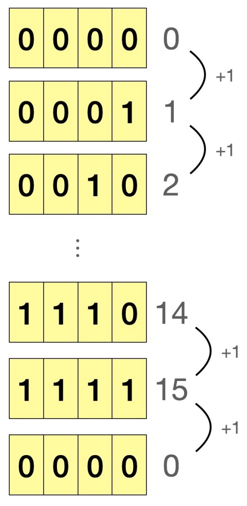
If we consider the case of a 4-bit binary, and start counting from 0, the maximum number we can possibly represent is 15. Adding 1 to 15, would lead to 0 being represented, as shown in Figure 1. This is called integer overflow, just like how an old car’s analogue 4-digit odometer “resets” to zero after recording 9999 km. As for the problem of running the same code and getting different results on a Windows and Mac machine, a numpy integer array on Windows defaults to 32-bit integer, whereas it is 64-bit on Mac/Linux, and as expected, the 64-bit integer has more bits and can thus represent our expected value of 5000050000. So, how do we mitigate this problem when writing future code? Simply specify the type argument and force Python to use 64-bit integers when needed.

>>> hard_sum = np.sum(np.arange(1,100001), dtype=np.int64)
>>> print(type(hard_sum))
<class 'numpy.int64'>
>>> print(hard_sum)
5000050000

As to why we got the spurious value of 705082704 from using 32-bit integers, I will leave it to you to understand it from the second edition of my book, Python Puzzlers!

Figure 1: Illustration of overflow in a 4-bit unsigned integer

Example #2: An Important Pointer for Copying Things

Antonio: On to another simple example, numpy arrays! Consider the following two-dimensional array of temperatures in degree Celsius.

>>> t_degrees_original = np.array([[2,1,0,1], [-1,0,-1,-1], [-3,-5,-2,-3], [-5,-7,-6,-7]])

Antonio: Let’s say we only want the first three rows of data, and in this selection would like to set all values on the zeroth row to zero, while retaining the values in the original array. Any ideas how we could do that?

Cecilio: Hey! I’ve learnt this last term, we do array slicing.

>>> t_degrees_slice = t_degrees_original[0:3,:]
>>> t_degrees_slice[0,:] = 0

Antonio: I did say to retain the values in the original array…

>>> print(t_degrees_original)
[[ 0  0  0  0]
[-1  0 -1 -1]
[-3 -5 -2 -3]
[-5 -7 -6 -7]]

Cecilio: Oh oops.

Berenice: Let me suggest a better solution.

>>> t_degrees_original = np.array([[2,1,0,1], [-1,0,-1,-1], [-3,-5,-2,-3], [-5,-7,-6,-7]])
>>> t_degrees_slice = t_degrees_original[[0,1,2],:]
>>> t_degrees_slice[0,:] = 0
>>> print(t_degrees_original)
[[ 2  1  0  1]
[-1  0 -1 -1]
[-3 -5 -2 -3]
[-5 -7 -6 -7]]

Antonio: Well done!

Cecilio: What? I thought the array indices 0:3 and 0,1,2 would give you the same slice of the numpy array.

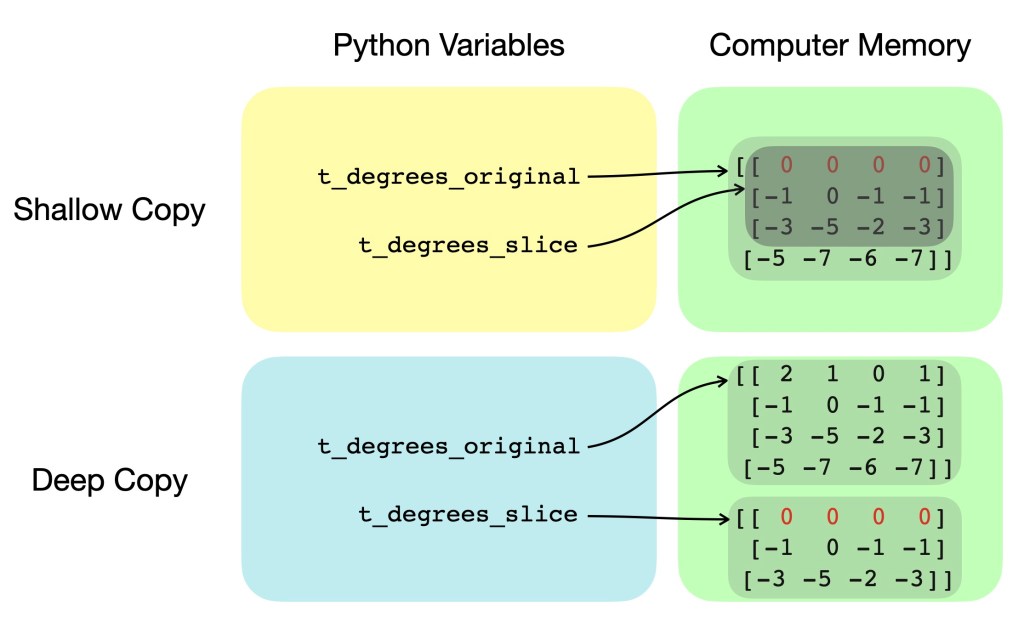
Antonio: Let’s clarify this. The former method of using 0:3 is standard indexing and only copies the information on where the original array was stored (i.e. “view” of the original array, or “shallow copy”), while the latter 0,1,2 is fancy indexing and actually makes a new separate array with the corresponding values from the original array (i.e. “deep copy”). This is illustrated in Figure 2 showing variables and their respective pointers for both shallow and deep copying. As you now understand, numpy, is really not as easy as pie…

Figure 2: Simplified diagram showing differences in variable pointers and computer memory for shallow and deep copying

Cecilio: That was… deep.

Berenice: Is there a better way to deep copy numpy arrays rather than having to type in each index like I did e.g. [0,1,2]?

Antonio: There is definitely a better way! If we replace the first line of your code with the line below, you should be able to do a deep copy of the original array. Editing the copied array will not affect the original array.

>>> t_degrees_slice = np.copy(t_degrees_original[0:2,:])

I would suggest this method of np.copy to be your one– and preferably only one –obvious way to do a deep copy of a numpy array, since it’s the most intuitive and human-readable! But remember, deep copy only if you have to, since deep copying a whole array of values takes computation time and space! It’s now time for a 5-minute break.

Cecilio: More like time for me to eat some humble (num)py.

Antonio: Hope you all had a nice break. We now start with a fun pop quiz!

short_a = "galileo galilei"
short_b = "galileo galilei"
long_a = "galileo galilei " + "linceo"
long_b = "galileo galilei " + "linceo"
 
print(short_a == short_b)
print(short_a is short_b)
print(long_a == long_b)
print(long_a is long_b)

Antonio: In fact, they are all correct answers. It depends on whether you are running Python 3.6.0, Python 3.8.5 and whether you ran the code in a script or in the console! Although there is much more to learn about “string interning”, the quick lesson here is to always compare the value of strings using double equal signs (==) instead of using is.

Example #3: Array manipulation – A Sleight of Hand?

Antonio: Let’s say you are asked to calculate the centered difference of some quantity (e.g. temperature) in one dimension with gird points uniformly separated by of 1 metre. What is some code that we could use to do this?

Berenice: I remember this from one of the modelling courses. We could use a for loop to calculate most elements of then deal with the boundary conditions. The code may look something like this:

delta_x = 1.0
temp_x = np.random.rand(1000)
dtemp_dx = np.empty_like(temp_x)
for i in range(1, len(temp_x)-1):
    dtemp_dx[i] = (temp_x[i+1] - temp_x[i-1]) / (2*delta_x)

# Boundary conditions
dtemp_dx[0] = dtemp_dx[1]
dtemp_dx[-1] = dtemp_dx[-2]

Antonio: Right! How about we replace your for loop with this line?

dtemp_dx[1:-1] = (temp_x[2:] - temp_x[0:-2]) / (2*delta_x)

Cecilio: Don’t they just do the same thing?

Antonio: Yes, but would you like to have a guess which one might be the “better” way?

Berenice: In last term’s modules, we were only taught the method I proposed just now. I would have thought both methods were equally good.

Antonio: On my computer, running your version of code 10000 times takes 6.5 seconds, whereas running my version 10000 times takes 0.1 seconds.

Cecilio: That was… fast!

Berenice: Only if my research code could run with that kind of speed…

Antonio: And that is what we call vectorisation, the act of taking advantage of numpy’s optimised loop implementation instead of having to write your own!

Cecilio: I wish we knew all this earlier on! Can you tell us more?

Antonio: Glad your interest is piqued! Anyway, that’s all the time we have today. For this week’s homework, please familiarise yourself so you know how to

import this

module or import that package. In the next few lectures, we will look at more bewildering behaviours such as the “Mesmerising Mutation”, the “Out of Scope” problem that is in the scope of this module. As we move to more advanced aspects of this course, we may even come across the “Dynamic Duck” and “Mischievous Monkey”. Bye for now!