The importance of anticyclonic synoptic eddies for atmospheric block persistence and forecasts

Charlie Suitters – c.c.suitters@pgr.reading.ac.uk

The Beast from the East, the record-breaking winter warmth of February 2020, the Canadian heat dome of 2022…what do these three events have in common? Well, many things I’m sure, but most relevantly for this blog post is that they all coincided with the same phenomenon – atmospheric blocking.

So what exactly is a block? An atmospheric block is a persistent, large-scale, quasi-stationary high-pressure system sometimes found in the mid-latitudes. The prolonged subsidence associated with the high pressure suppresses cloud formation, therefore blocks are often associated with clear, sunny skies, calm winds, and temperature extremes. Their impacts can be diverse, including both extreme heat and extreme cold, drought, poor air quality, and increased energy demand (Kautz et al., 2022). 

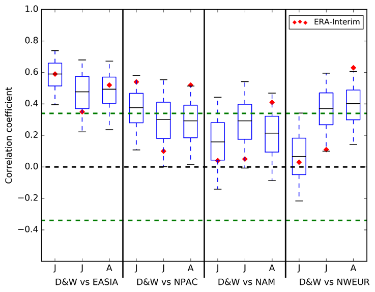
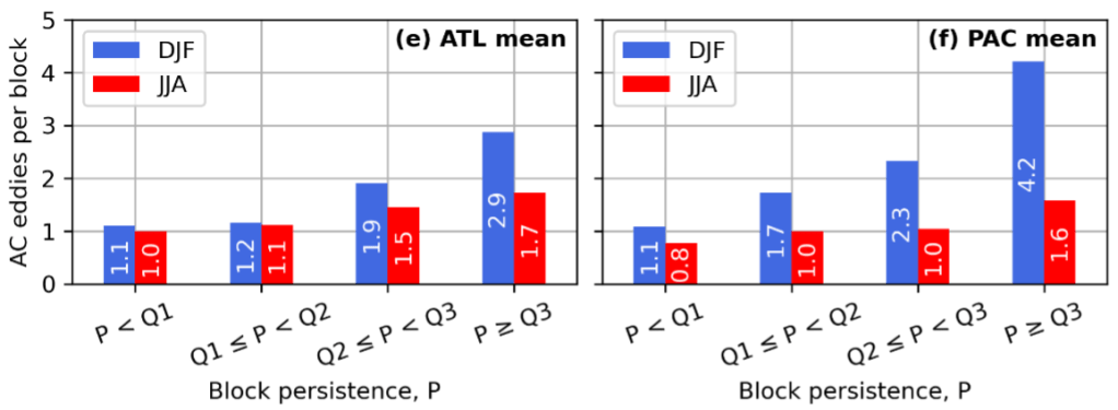
Despite the range of hazards that blocking can bring, we still do not fully understand the dynamics that cause a block to start, maintain itself, and decay (Woollings et al., 2018). In reality, many different mechanisms are at play, but the importance of each process can vary between location, season, and individual block events (Miller and Wang, 2022). One process that is known to be important is the interaction between blocks and smaller synoptic-scale transient eddies (Shutts, 1983; Yamazaki and Itoh, 2013). By studying a 43-year climatology of atmospheric blocks and their anticyclonic eddies (both defined by regions of anomalously high 500 hPa geopotential height), I have found that on average, longer blocks absorb more synoptic anticyclones, which “tops up their anticyclonicness” and allows them to persist longer (Fig. 1).

Figure 1: average number of anticyclonic eddies per block for the Euro-Atlantic (left) and North Pacific (right). Block persistence is defined as the quartiles (Q1, Q2, Q3) of all blocks in winter (blue) and summer (red). From Suitters et al. (2023).

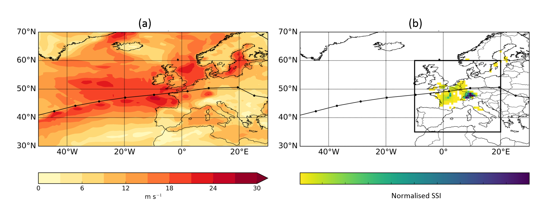
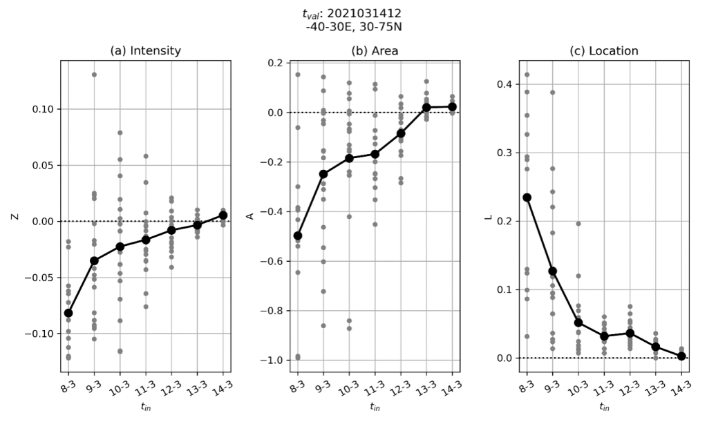
It’s great that we now know this relationship, however it would be beneficial to know if these interactions are forecasted well. If they are not, it might explain our shortcomings in predicting the longevity of a block event (Ferranti et al., 2015).  I explore this with a case study from March 2021 using ensemble forecasts from MOGREPS-G. Fortunately, this block in March 2021 was not associated with any severe weather, but it was still not forecasted well. In Figure 2, I show normalised errors in the strength, size, and location of the block, at the time of block onset, for each ensemble member from a range of different initialisation times. In these plots, a negative (positive) value means that the block was forecast to be too weak (strong) or too small (large), and the larger the error in the location, the further away the forecast block was from reality. In general, the onset of this block was forecast to be to be too weak and too small, though there was considerable spread within the ensemble (Fig. 2). Certainty in the forecast was only achieved at relatively small lead times.

Figure 2: Normalised errors in the intensity (left), area (centre), and location of the block’s centre of mass (right), at a validity time of 2021-03-14 12 UTC (the time of onset). Each ensemble member’s error from a particular initialisation time is shown by the grey dots, and the ensemble mean is shown in black. When Z, A, or L are zero, the forecast has a “perfect” replication for this metric of the block (when compared to ERA5 reanalysis).

Now for the interesting bit – what causes the uncertainty in forecasting of the onset this European blocking event? To examine this, I grouped forecast members from an initialisation time of 8 March 2021 according to their ability to replicate the real block: the entire MOGREPS-G mean, members that either have no block or a very small block (Group G), members that perform best (Group H), and members that predict area well, but have the block in the wrong location (Group I). Then, I take the mean geopotential height anomalies () at each time step in each group, and compare these fields between groups to see if I can find a source of forecast error.

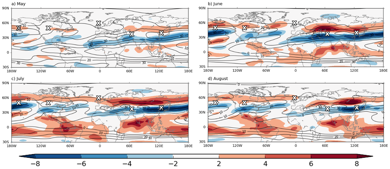
This is shown as an animation in Fig. 3. The animation starts at the time of block onset, and goes back in time to selected validity times, as shown at the top of the figure. The domain of the plot also changes in each frame, gradually moving westwards across the Atlantic. By looking at the ERA5 (the “real”) evolution of the block, we see that the onset of the European block was the result of an anticyclonic transient eddy breaking off from an upstream blocking event over North America. However, none of the aforementioned groups of members accurately simulate this vortex shedding from the North American block. In most cases, the eddy leaving the North American block is either too weak or non-existent (as shown by the blue shading, representing that the forecast is much weaker than in ERA5), which resulted in a lack of Eastern Atlantic blocking altogether. Only the group that modelled the block well (Group H) had a sizeable eddy breaking off from the upstream block, but even in this case it was too weak (paler blue shading). Therefore, the uncertain block onset in this case is directly related to the way in which an anticyclonic eddy was forecast to travel (or not) across the Atlantic, from a pre-existing block upstream. This is interesting because the North American block itself was modelled well, yet the eddy that broke off it was not, which was vital for the onset of the Euro-Atlantic block.

To conclude, this is an important finding because it shows the need to accurately model synoptic-scale features in the medium range in order to accurately predict blocking. If these eddies are absent in a forecast, a block might not even form (as I have shown), and therefore potentially hazardous weather conditions would not be forecast until much shorter lead times. My work shows the role of anticyclonic eddies towards the persistence and forecasting of blocks, which until now had not be considered in detail.

References

Kautz, L., Martius, O., Pfahl, S., Pinto, J.G., Ramos, A.M., Sousa, P.M., and Woollings, T., 2022. “Atmospheric blocking and weather extremes over the Euro-Atlantic sector–a review.” Weather and climate dynamics, 3(1), pp305-336.

Miller, D.E. and Wang, Z., 2022. Northern Hemisphere winter blocking: differing onset mechanisms across regions. Journal of the Atmospheric Sciences, 79(5), pp.1291-1309.

Shutts, G.J., 1983. The propagation of eddies in diffluent jetstreams: Eddy vorticity forcing of ‘blocking’ flow fields. Quarterly Journal of the Royal Meteorological Society, 109(462), pp.737-761.

Suitters, C.C., Martínez-Alvarado, O., Hodges, K.I., Schiemann, R.K. and Ackerley, D., 2023. Transient anticyclonic eddies and their relationship to atmospheric block persistence. Weather and Climate Dynamics, 4(3), pp.683-700.

Woollings, T., Barriopedro, D., Methven, J., Son, S.W., Martius, O., Harvey, B., Sillmann, J., Lupo, A.R. and Seneviratne, S., 2018. Blocking and its response to climate change. Current climate change reports, 4, pp.287-300.

Yamazaki, A. and Itoh, H., 2013. Vortex–vortex interactions for the maintenance of blocking. Part I: The selective absorption mechanism and a case study. Journal of the Atmospheric Sciences, 70(3), pp.725-742.

Fluid Dynamics Summer School 

Charlie Suitters – c.c.suitters@pgr.reading.ac.uk 

Every year, Cambridge and École Polytechnique in Paris alternate hosting duties of the Fluid Dynamics of Sustainability and the Environment (FDSE) summer school. This ran for two weeks earlier in September, and like many other things took place online. After talking to previous attendees of the summer school, I went into the fortnight with excitement but also trepidation, as I had heard that it has an intense programme! Here is my experience of a thoroughly enjoyable couple of weeks. 

Structure 

The summer school brought together around 50 PhD students and a few postdocs from all over the world, from Japan to Europe to Arizona, and I have to admire the determination of those students who attended the school at unsociable times of the day! We all came from different backgrounds – some had a meteorological background like myself, but there were also oceanographers, fluid dynamicists, engineers and geographers to name but a few. It was great to hear from so many students who are passionate about their work in two brief ice-breaker sessions where we introduced ourselves to the group and I got to appreciate how wide-reaching the FDSE community is. 

Each day consisted of four 1-hour lectures – normally three ‘core’ subjects (fluid dynamics basics, atmospheric dynamics, climate, oceanography, etc.) and one guest lecturer per day (including our very own Sue Gray who gave us a whistle-stop tour of the mesoscale and extratropical cyclones). After this, there was the opportunity to split into breakout groups and speak to the day’s lecturers to ask them questions and spark discussions in small groups. On the final day, we also had a virtual tour of the various fluid dynamics labs that Cambridge has (there are a lot!) and a few of the students in the labs spoke about their work. 

Core Lectures 

Figure 1. Demonstration of a density current (blue) of salty water in a tank of less dense tap water. Taken from Jean-Marc Chomaz’s lecture

These lectures were given by very engaging specialists including Colm-Cille Caulfield, John Taylor, Alison Ming, Jerome Neufeld and Jean-Marc Chomaz; and provided the perfect opportunity to see lots of pretty videos about fluid flows (Fig. 1). Having done an undergraduate course in Meteorology, a lot of these gave me a refresher of things I should already know, but it was refreshing to see how other lecturers approach the same material. 

The most interesting core lectures to me were those regarding renewable energy, given by Riwal Plougonuen and Alex Stegner. Plougonuen lectured us on wind turbines, telling us how they worked and why they are designed like they are – did you know that actually the most efficient wind turbines have 2 blades, but the vast majority have three for better structural stability? On the other hand, Stegner spoke to us about hydroelectricity, and I learned that Norway produces nearly all of its electricity through hydropower. Other highlights from these core lectures include watching a video of a research hut being swamped by an avalanche (Nathalie Vriend, see video at the link here), and seeing Jerome Neufeld demonstrate ice flows using golden syrup (he likes his food!) 

Guest Lectures 

Figure 2. Flow patterns around a sash window with both slots open – the blue arrows showing incoming cold air and the red arrows showing warm flow to the outside. Taken from Megan Davies Wykes’ lecture.

For me, the guest lectures were the highlights of my time at the summer school. These lectures often explored things beyond my area of expertise, and demonstrated just how the fluid mechanics we had learned are highly applicable to many different areas of life. We had a lecture about building ventilation from Megan Davies Wykes, which made me realise that adequately ventilating a room is more than simply cracking open a window – you have to consider everything from the size of the room, outside wind speed, how many windows there are, and even the body heat from people inside the room. Davies Wykes’s passion about people using their sash windows correctly will always stick with me – turns out you need to open both the top and the bottom panes for the best ventilation (something she emphasised more than once!), see Fig. 2.  

Figure 3. Demonstration of how droplets and plumes of air from the mouth are kept closer to the body when wearing a mask (Bhagat et al. 2020).

Fittingly, we also had a lecture from Paul Linden about the transmission of Covid, and he demonstrated how effective masks are at preventing transmission using a great visualisation (Fig. 3). It was great to have topics such as these that are relevant in today’s world, and provided yet another real-world application of the fluid dynamics we had learned. 

Breakout Discussion Sessions 

Every afternoon, the day’s lecturers returned and invited us to ask them questions about their lectures, or just have an intelligent discussion about their area of expertise. Admittedly these sessions could get a little awkward when everyone was too tired to ask anything towards the end of the long two weeks, but these sessions were still incredibly useful. They provided us the means to speak to a professional in their field about their research, and allowed us time to network and ask them some challenging questions. 

Concluding Remarks 

Of course, over the course of the two weeks we learned so much more than what I described above, and yet again demonstrates the versatility of the field! The summer school as a whole was organised really well and the lecturers were engaging and genuinely interested in hearing about us and our projects. I would highly recommend attending this summer school next year to any PhD student – the scope of the school was so broad that I am sure there will be something for everyone in the programme, and fingers crossed it goes ahead in Paris next year! 

References 

Bhagat, R., Davies Wykes, M., Dalziel, S., & Linden, P. (2020). Effects of ventilation on the indoor spread of COVID-19. Journal of Fluid Mechanics, 903, F1. doi:10.1017/jfm.2020.720 

The effect of surface heat fluxes on the evolution of storms in the North Atlantic storm track

Andrea Marcheggiani – a.marcheggiani@pgr.reading.ac.uk

Diabatic processes are typically considered as a source of energy for weather systems and as a primary contributing factor to the maintenance of mid-latitude storm tracks (see Hoskins and Valdes 1990 for some classical reading, but also a more recent reviews, e.g. Chang et al. 2002). However, surface heat exchanges do not necessarily act as a fuel for the evolution of weather systems: the effects of surface heat fluxes and their coupling with lower-tropospheric flow can be detrimental to the potential energy available for systems to grow. Indeed, the magnitude and sign of their effects depend on the different time (e.g., synoptic, seasonal) and length (e.g., global, zonal, local) scales which these effects unfold at.


Figure 1: Composites for strong (a-c) and weak (d-f) values of the covariance between heat flux and temperature time anomalies.

Heat fluxes arise in response to thermal imbalances which they attempt to neutralise. In the atmosphere, the primary thermal imbalances that are observed correspond with the meridional temperature gradient caused by the equator—poles differential radiative heating from the Sun, and the temperature contrasts at the air—sea interface which essentially derives from the different heat capacities of the oceans and the atmosphere.

In the context of the energetic scheme of the atmosphere, which was first formulated by Lorenz (1955) and commonly known as Lorenz energy cycle, the meridional transport of heat (or dry static energy) is associated with conversion of zonal available potential energy to eddy available potential energy, while diabatic processes at the surface coincide with generation of eddy available potential energy.

Figure 2: Phase portrait of FT covariance and mean baroclinicity. Streamlines indicate average circulation in the phase space (line thickness proportional to phase speed). The black shaded dot in the top left corner indicates the size of the Gaussian kernel used in the smoothing process. Colour shading indicates the number of data points contributing to the kernel average

The sign of the contribution from surface heat exchanges to the evolution on weather systems is not univocal, as it depends on the specific framework which is used to evaluate their effects. Globally, these have been estimated to have a positive effect on the potential energy budget (Peixoto and Oort, 1992) while locally the picture is less clear, as heating where it is cold and cooling where it is warm would lead to a reduction in temperature variance, which is essentially available potential energy.

The first part of my PhD focussed on assessing the role of local air—sea heat exchanges on the evolution of synoptic systems. To that extent, we built a hybrid framework where the spatial covariance between time anomalies of sensible heat flux F and lower-tropospheric air temperature T  is taken as a measure of the intensity of the air—sea thermal coupling. The time anomalies, denoted by a prime, are defined as departures from a 10-day running mean so that we can concentrate on synoptic variability (Athanasiadis and Ambaum, 2009). The spatial domain where we compute the spatial covariance extends from 30°N to 60°N and from 30°W to 79.5°W, which corresponds with the Gulf Stream extension region, and to focus on air—sea interaction, we excluded grid points covered by land or ice.

This leaves us with a time series for F’—T’ spatial covariance, which we also refer to as FT index.

The FT index is found to be always positive and characterised by frequent bursts of intense activity (or peaks). Composite analysis, shown in Figure 1 for mean sea level pressure (a,d), temperature at 850hPa (b,e) and surface sensible heat flux (c,f), indicates that peaks of the FT index (panels a—c) correspond with intense weather activity in the spatial domain considered (dashed box in Figure 1) while a more settled weather pattern is observed to be typical when the FT index is weak (panels d—f).


Figure 3: Phase portraits for spatial-mean T (a) and cold sector area fraction (b). Shading in (a) represents the difference between phase tendency and the mean value of T, as reported next to the colour bar. Arrows highlight the direction of the circulation, kernel-averaged using the Gaussian kernel shown in the top-left corner of each panel.

We examine the dynamical relationship between the FT index and the area-mean baroclinicity, which is a measure of available potential energy in the spatial domain. To do that, we construct a phase space of FT index and baroclinicity and study the average circulation traced by the time series for the two dynamical variables. The resulting phase portrait is shown in Figure 2. For technical details on phase space analysis refer to Novak et al. (2017), while for more examples of its use see Marcheggiani and Ambaum (2020) or Yano et al. (2020). We observe that, on average, baroclinicity is strongly depleted during events of strong F’—T’ covariance and it recovers primarily when covariance is weak. This points to the idea that events of strong thermal coupling between the surface and the lower troposphere are on average associated with a reduction in baroclinicity, thus acting as a sink of energy in the evolution of storms and, more generally, storm tracks.

Upon investigation of the driving mechanisms that lead to a strong F’—T’ spatial covariance, we find that increases in variances and correlation are equally important and that appears to be a more general feature of heat fluxes in the atmosphere, as more recent results appear to indicate (which is the focus of the second part of my PhD).

In the case of surface heat fluxes, cold sector dynamics play a fundamental role in driving the increase of correlation: when cold air is advected over the ocean surface, flux variance amplifies in response to the stark temperature contrasts at the air—sea interface as the ocean surface temperature field features a higher degree of spatial variability linked to the presence of both the Gulf Stream on the large scale and oceanic eddies on the mesoscale (up to 100 km).

The growing relative importance of the cold sector in the intensification phase of the F’—T’ spatial covariance can also be revealed by looking at the phase portraits for air temperature and cold sector area fraction, which is shown in Figure 3. These phase portraits tell us how these fields vary at different points in the phase space of surface heat flux and air temperature spatial standard deviations (which correspond to the horizontal and vertical axes, respectively). Lower temperatures and larger cold sector area fraction characterise the increase in covariance, while the opposite trend is observed in the decaying stage.

Surface heat fluxes eventually trigger an increase in temperature variance, which within the atmospheric boundary layer follows an almost adiabatic vertical profile which is characteristic of the mixed layer (Stull, 2012).

Figure 4: Diagram of the effect of the atmospheric boundary layer height on modulating surface heat flux—temperature correlation.

Stronger surface heat fluxes are associated with a deeper boundary layer reaching higher levels into the troposphere: this could explain the observed increase in correlation as the lower-tropospheric air temperatures become more strongly coupled with the surface, while a lower correlation with the surface ensues when the boundary layer is shallow and surface heat flux are weak. Figure 4 shows a simple diagram summarising the mechanisms described above.

In conclusion, we showed that surface heat fluxes locally can have a damping effect on the evolution of mid-latitude weather systems, as the covariation of surface heat flux and air temperature in the lower troposphere corresponds with a decrease in the available potential energy.

Results indicate that most of this thermodynamically active heat exchange is realised within the cold sector of weather systems, specifically as the atmospheric boundary layer deepens and exerts a deeper influence upon the tropospheric circulation.

References

  • Athanasiadis, P. J. and Ambaum, M. H. P.: Linear Contributions of Different Time Scales to Teleconnectivity, J. Climate, 22, 3720– 3728, 2009.
  • Chang, E. K., Lee, S., and Swanson, K. L.: Storm track dynamics, J. Climate, 15, 2163–2183, 2002.
  • Hoskins, B. J. and Valdes, P. J.: On the existence of storm-tracks, J. Atmos. Sci., 47, 1854–1864, 1990.
  • Lorenz, E. N.: Available potential energy and the maintenance of the general circulation, Tellus, 7, 157–167, 1955.
  • Marcheggiani, A. and Ambaum, M. H. P.: The role of heat-flux–temperature covariance in the evolution of weather systems, Weather and Climate Dynamics, 1, 701–713, 2020.
  • Novak, L., Ambaum, M. H. P., and Tailleux, R.: Marginal stability and predator–prey behaviour within storm tracks, Q. J. Roy. Meteorol. Soc., 143, 1421–1433, 2017.
  • Peixoto, J. P. and Oort, A. H.: Physics of climate, American Institute of Physics, New York, NY, USA, 1992.
  • Stull, R. B.: Mean boundary layer characteristics, In: An Introduction to Boundary Layer Meteorology, Springer, Dordrecht, Germany, 1–27, 1988.
  • Yano, J., Ambaum, M. H. P., Dacre, H., and Manzato, A.: A dynamical—system description of precipitation over the tropics and the midlatitudes, Tellus A: Dynamic Meteorology and Oceanography, 72, 1–17, 2020.

The Circumglobal Teleconnection and its Links to Seasonal Forecast Skill for the European Summer

Email: j.beverley@pgr.reading.ac.uk

Recent extreme weather events such as the central European heatwave in 2003, flooding in the UK in 2007, and even the recent dry summer in the UK in 2018, have highlighted the need for more accurate long-range forecasts for the European summer. Recent research has led to improvements in European winter seasonal forecasts, however summer forecast skill remains relatively low. One potential source of predictability for Europe is the Indian summer monsoon, which can affect European weather via a global wave train known as the “Circumglobal Teleconnection” (CGT).

figure1
Figure 1: One-point correlation between 200 hPa geopotential height at the base point (35°-40°N, 60°-70°E) and 200 hPa geopotential height elsewhere in the ERA-Interim (1981–2014) reanalysis dataset, for August. The boxes indicate the regions defined as the “centres of action” of the CGT – these are North Pacific (NPAC), North America (NAM), Northwest Europe (NWEUR), Ding and Wang (D&W) and East Asia (EASIA).

The CGT was first identified by Ding and Wang (2005) as having a major role in modulating observed weather patterns in the Northern Hemisphere summer. Using a 200 hPa geopotential height index centred in west-central Asia (35°-40°N, 60°-70°E), they constructed a one-point correlation map of geopotential height with reference to this index (reproduced in Figure 1). From this, they identified a wavenumber-5 structure where the pressure variations over the Northeast Atlantic, East Asia, North Pacific and North America are all nearly in phase with the variations over west-central Asia (these are known as the “centres of action”). They also showed that the CGT is associated with significant temperature and precipitation anomalies in Europe, so accurate representation this mechanism in seasonal forecast models could provide an important source of subseasonal to seasonal forecast skill.

The model used here is a version of the European Centre for Medium-Range Weather Forecasts (ECMWF)’s coupled seasonal forecast model. Reforecasts are initialised on 1st May and are run for four months, so cover May-August, with start dates from 1981-2014. The skill of the model 200 hPa geopotential height is shown in Figure 2, defined as the correlation between the model ensemble mean and ERA-Interim. The model has good skill in May (to be expected given that the reforecasts are initialised in May) but in June, July and August areas of zero or negative correlation develop across much of the northern hemisphere extratropics. The areas of reduced skill align closely with the location of the centres of action of the CGT shown in Figure 1, suggesting that there is a link between the model skill and the model representation of the CGT.

figure2
Figure 2: Model ensemble mean skill for 200 hPa geopotential height as defined as the correlation between ERA-Interim and model ensemble mean for (a) May (b) June (c) July and (d) August

To determine how well the model represents the CGT, Figure 3 shows the correlation between the D&W region and the other centres of action of the CGT, as defined in Figure 1. Focussing on August (as August has the strongest CGT pattern) it can be seen that the model correlations, indicated by the box and whisker plots, are weaker than in observations (red diamond) for the D&W vs. North Pacific (NPAC), North America (NAM) and Northwest Europe (NWEUR) regions. This indicates that the model has a weak representation of the wavetrain associated with the CGT.

figure3
Figure 3: Distribution of correlation coefficients for the D&W Index correlated against the other centres of action of the CGT. The box plots represent the upper and lower quartiles, and the whiskers extend to the 5th and 95th percentiles. The black horizontal line represents the median value and the red diamond the observed correlation coefficient from ERA-Interim.

There are likely to be several reasons for the weak representation of the CGT in the model. One important factor is the presence of a northerly jet bias in the model across much of the Northern Hemisphere. This can be seen in Figure 4, which shows the model jet biases relative to ERA-Interim in the coloured contours, and the observed zonal wind in the black contours. The dipole structure of the biases which exists across much of the hemisphere, particularly in June, July and August, indicates that the model jet stream is located too far to the north. This means that Rossby waves forced in this region will have different wave propagation characteristics to reality – they may propagate at the incorrect speed, in the wrong direction or may not propagate at all, and this is likely to be an important factor in the weak representation of the CGT in the model.

figure4
Figure 4: Model 200 hPa zonal wind bias (filled contours, m/s), defined as the model ensemble mean minus ERA-Interim zonal wind, and ERA-I 200 hPa zonal wind (black contours) for (a) May (b) June (c) July and (d) August. The location of the centres of action of the CGT are marked with white crosses.

Other potential factors involved are a poor representation of the link between monsoon precipitation and the geopotential height in west-central Asia (which was shown by Ding and Wang (2007) to be important in the maintenance of the CGT) and errors in the forcing of Rossby waves associated with the monsoon. For a more detailed explanation of these, see my paper in Climate Dynamics (Beverley et al. 2018). It seems likely that the pattern of reduced skill in Figure 2, with negative correlations located at the centres of action of the CGT, including over Europe, is related to the poor representation of the CGT in the model. This raises the question of whether an improvement in the model’s representation of the CGT would lead to an improvement in forecast skill for the European summer. To address this question, sensitivity experiments have been carried out, in which the observed circulation is imposed in several centres of action along the CGT pathway to explore the impact on forecast skill for European summer weather.

References

Beverley, J. D., S. J. Woolnough, L. H. Baker, S. J. Johnson and A. Weisheimer, 2018: The northern hemisphere circumglobal teleconnection in a seasonal forecast model and its relationship to European summer forecast skill. Clim. Dyn. https://doi.org/10.1007/s00382-018-4371-4

Ding, Q., and B. Wang, 2005: Circumglobal teleconnection in the northern hemisphere summer. J. Clim. 18, 3483–3505.  https://doi.org/10.1175/JCLI3473.1

Ding, Q., and B. Wang, 2007: Intraseasonal teleconnection between the summer Eurasian wave train and the Indian monsoon. J. Clim. 20, 3751-3767. https://doi.org/10.1175/JCLI4221.1

Modelling windstorm losses in a climate model

Extratropical cyclones cause vast amounts of damage across Europe throughout the winter seasons. The damage from these cyclones mainly comes from the associated severe winds. The most intense cyclones have gusts of over 200 kilometres per hour, resulting in substantial damage to property and forestry, for example, the Great Storm of 1987 uprooted approximately 15 million trees in one night. The average loss from these storms is over $2 billion per year (Schwierz et al. 2010) and is second only to Atlantic Hurricanes globally in terms of insured losses from natural hazards. However, the most severe cyclones such as Lothar (26/12/1999) and Kyrill (18/1/2007) can cause losses in excess of $10 billion (Munich Re, 2016). One property of extratropical cyclones is that they have a tendency to cluster (to arrive in groups – see example in Figure 1), and in such cases these impacts can be greatly increased. For example Windstorm Lothar was followed just one day later by Windstorm Martin and the two storms combined caused losses of over $15 billion. The large-scale atmospheric dynamics associated with clustering events have been discussed in a previous blog post and also in the scientific literature (Pinto et al., 2014; Priestley et al. 2017).

Picture1
Figure 1. Composite visible satellite image from 11 February 2014 of 4 extratropical cyclones over the North Atlantic (circled) (NASA).

A large part of my PhD has involved investigating exactly how important the clustering of cyclones is on losses across Europe during the winter. In order to do this, I have used 918 years of high resolution coupled climate model data from HiGEM (Shaffrey et al., 2017) which provides a huge amount of winter seasons and cyclone events for analysis.

In order to understand how clustering affects losses, I first of all need to know how much loss/damage is associated with each individual cyclone. This is done using a measure called the Storm Severity Index (SSI – Leckebusch et al., 2008), which is a proxy for losses that is based on the 10-metre wind field of the cyclone events. The SSI is a good proxy for windstorm loss. Firstly, it scales the wind speed in any particular location by the 98th percentile of the wind speed climatology in that location. This scaling ensures that only the most severe winds at any one point are considered, as different locations have different perspectives on what would be classed as ‘damaging’. This exceedance above the 98th percentile is then raised to the power of 3 due to damage from wind being a highly non-linear function. Finally, we apply a population density weighting to our calculations. This weighting is required because a hypothetical gust of 40 m/s across London will cause considerably more damage than the same gust across far northern Scandinavia, and the population density is a good approximation for the density of insured property. An example of the SSI that has been calculated for Windstorm Lothar is shown in Figure 2.


figure_2_blog_2018_new
Figure 2. (a) Wind footprint of Windstorm Lothar (25-27/12/1999) – 10 metre wind speed in coloured contours (m/s). Black line is the track of Lothar with points every 6 hours (black dots). (b) The SSI field of Windstorm Lothar. All data from ERA-Interim.


From Figure 2b you can see how most of the damage from Windstorm Lothar was concentrated across central/northern France and also across southern Germany. This is because the winds here were most extreme relative to what is the climatology. Even though the winds are highest across the North Atlantic Ocean, the lack of insured property, and a much high climatological winter mean wind speed, means that we do not observe losses/damage from Windstorm Lothar in these locations.

figure_3_blog_2018_new
Figure 3. The average SSI for 918 years of HiGEM data.


I can apply the SSI to all of the individual cyclone events in HiGEM and therefore can construct a climatology of where windstorm losses occur. Figure 3 shows the average loss across all 918 years of HiGEM. You can see that the losses are concentrated in a band from southern UK towards Poland in an easterly direction. This mainly covers the countries of Great Britain, Belgium, The Netherlands, France, Germany, and Denmark.

This blog post introduces my methodology of calculating and investigating the losses associated with the winter season extratropical cyclones. Work in Priestley et al. (2018) uses this methodology to investigate the role of clustering on winter windstorm losses.

This work has been funded by the SCENARIO NERC DTP and also co-sponsored by Aon Benfield.


Email: m.d.k.priestley@pgr.reading.ac.uk


References

Leckebusch, G. C., Renggli, D., and Ulbrich, U. 2008. Development and application of an objective storm severity measure for the Northeast Atlantic region. Meteorologische Zeitschrift. https://doi.org/10.1127/0941-2948/2008/0323.

Munich Re. 2016. Loss events in Europe 1980 – 2015. 10 costliest winter storms ordered by overall losses. https://www.munichre.com/touch/naturalhazards/en/natcatservice/significant-natural-catastrophes/index.html

Pinto, J. G., Gómara, I., Masato, G., Dacre, H. F., Woollings, T., and Caballero, R. 2014. Large-scale dynamics associated with clustering of extratropical cyclones affecting Western Europe. Journal of Geophysical Research: Atmospheres. https://doi.org/10.1002/2014JD022305.

Priestley, M. D. K., Dacre, H. F., Shaffrey, L. C., Hodges, K. I., and Pinto, J. G. 2018. The role of European windstorm clustering for extreme seasonal losses as determined from a high resolution climate model, Nat. Hazards Earth Syst. Sci. Discuss., https://doi.org/10.5194/nhess-2018-165, in review.

Priestley, M. D. K., Pinto, J. G., Dacre, H. F., and Shaffrey, L. C. 2017. Rossby wave breaking, the upper level jet, and serial clustering of extratropical cyclones in western Europe. Geophysical Research Letters. https://doi.org/10.1002/2016GL071277.

Schwierz, C., Köllner-Heck, P., Zenklusen Mutter, E. et al. 2010. Modelling European winter wind storm losses in current and future climate. Climatic Change. https://doi.org/10.1007/s10584-009-9712-1.

Shaffrey, L. C., Hodson, D., Robson, J., Stevens, D., Hawkins, E., Polo, I., Stevens, I., Sutton, R. T., Lister, G., Iwi, A., et al. 2017. Decadal predictions with the HiGEM high resolution global coupled climate model: description and basic evaluation, Climate Dynamics, https://doi.org/10.1007/s00382-016-3075-x.

The Role of the Cloud Radiative Effect in the Sensitivity of the Intertropical Convergence Zone to Convective Mixing

Email: j.f.talib@pgr.reading.ac.uk

Talib, J., S.J. Woolnough, N.P. Klingaman, and C.E. Holloway, 2018: The Role of the Cloud Radiative Effect in the Sensitivity of the Intertropical Convergence Zone to Convective Mixing. J. Climate, 31, 6821–6838, https://doi.org/10.1175/JCLI-D-17-0794.1

Rainfall in the tropics is commonly associated with the Intertropical Convergence Zone (ITCZ), a discontinuous line of convergence collocated at the ascending branch of the Hadley circulation, where strong moist convection leads to high rainfall. What controls the location and intensity of the ITCZ remains a fundamental question in climate science.

ensemble_precip_neat_thesis
Figure 1: Annual-mean, zonal-mean tropical precipitation (mm day-1) from Global Precipitation Climatology Project (GPCP, observations, solid black line) and CMIP5 (current coupled models) output. Dashed line indicates CMIP5 ensemble mean.

In current and previous generations of climate models, the ITCZ is too intense in the Southern Hemisphere, resulting in two annual-mean, zonal-mean tropical precipitation maxima, one in each hemisphere (Figure 1).  Even if we take the same atmospheric models and couple them to a world with only an ocean surface (aquaplanets) with prescribed sea surface temperatues (SSTs), different models simulate different ITCZs (Blackburn et al., 2013).

Within a climate model parameterisations are used to replace processes that are too small-scale or complex to be physically represented in the model. Parameterisation schemes are used to simulate a variety of processes including processes within the boundary layer, radiative fluxes and atmospheric chemistry. However my work, along with a plethora of others, shows that the representation of the ITCZ is sensitive to the convective parameterisation scheme (Figure 2a). The convective parameterisation scheme simulates the life cycle of clouds within a model grid-box.

Our method of showing that the simulated ITCZ is sensitive to the convective parameterisation scheme is by altering the convective mixing rate in prescribed-SST aquaplanet simulations. The convective mixing rate determines the amount of mixing a convective parcel has with the environmental air, therefore the greater the convective mixing rate, the quicker a convective parcel will become similar to the environmental air, given fixed convective parcel properties.

AEIprecipCREon
Figure 2: Zonal-mean, time-mean (a) precipitation rates (mm day-1}$) and (b) AEI (W m-2) in simulations where the convective mixing rate is varied.

In our study, the structure of the simulated ITCZ is sensitive to the convective mixing rate. Low convective mixing rates simulate a double ITCZ (two precipitation maxima, orange and red lines in Figure 2a), and high convective mixing rates simulate a single ITCZ (blue and black lines).

We then associate these ITCZ structures to the atmospheric energy input (AEI). The AEI is the amount of energy left in the atmosphere once considering the top of the atmosphere and surface energy budgets. We conclude, similar to Bischoff and Schneider, 2016, that when the AEI is positive (negative) at the equator, a single (double) ITCZ is simulated (Figure 2b). When the AEI is negative at the equator, energy is needed to be transported towards the equator for equilibrium. From a mean circulation perspective, this take place in a double ITCZ scenario (Figure 3). A positive AEI at the equator, is associated with poleward energy transport and a single ITCZ.

blog_figure_ITCZ_simulation
Figure 3: Schematic of a single (left) and double ITCZ (right). Blue arrows denote energy transport. In a single ITCZ scenario more energy is transported in the upper branches of the Hadley circulation, resulting in a net-poleward energy transport. In a double ITCZ scenario, more energy is transport equatorward than poleward at low latitudes, leading to an equatorward energy transport.

In our paper, we use this association between the AEI and ITCZ to hypothesize that without the cloud radiative effect (CRE), atmospheric heating due to cloud-radiation interactions, a double ITCZ will be simulated. We also hypothesize that prescribing the CRE will reduce the sensitivity of the ITCZ to convective mixing, as simulated AEI changes are predominately due to CRE changes.

In the rest of the paper we perform simulations with the CRE removed and prescribed to explore further the role of the CRE in the sensitivity of the ITCZ. We conclude that when removing the CRE a double ITCZ becomes more favourable and in both sets of simulations the ITCZ is less sensitive to convective mixing. The remaining sensitivity is associated with latent heat flux alterations.

My future work following this publication explores the role of coupling in the sensitivity of the ITCZ to the convective parameterisation scheme. Prescribing the SSTs implies an arbitary ocean heat transport, however in the real world the ocean heat transport is sensitive to the atmospheric circulation. Does this sensitivity between the ocean heat transport and atmospheric circulation affect the sensitivity of the ITCZ to convective mixing?

Thanks to my funders, SCENARIO NERC DTP, and supervisors for their support for this project.

References:

Blackburn, M. et al., (2013). The Aqua-planet Experiment (APE): Control SST simulation. J. Meteo. Soc. Japan. Ser. II, 91, 17–56.

Bischoff, T. and Schneider, T. (2016). The Equatorial Energy Balance, ITCZ Position, and Double-ITCZ Bifurcations. J. Climate., 29(8), 2997–3013, and Corrigendum, 29(19), 7167–7167.


Hierarchies of Models

With thanks to Inna Polichtchouk.

General circulation models (GCMs) of varying complexity are used in atmospheric and oceanic sciences to study different atmospheric processes and to simulate response of climate to climate change and other forcings.

However, Held (2005) warned the climate community that the gap between understanding and simulating atmospheric and oceanic processes is becoming wider. He stressed the use of model hierarchies for improved understanding of the atmosphere and oceans (Fig. 1). Often at the bottom of the hierarchy lie the well-understood, idealized, one- or two-layer models.  In the middle of the hierarchy lie multi-layer models, which omit certain processes such as land-ocean-atmosphere interactions or moist physics. And finally, at the top of the hierarchy lie fully coupled atmosphere-ocean general circulation models that are used for climate projections. Such model hierarchies are already well developed in other sciences (Held 2005), such as molecular biology, where studying less complex animals (e.g. mice) infers something about the more complex humans (through evolution).

Model_hierarchies_Shaw_etal2016
Figure 1: Model hierarchy of midlatitude atmosphere (as used for studying storm tracks). The simplest models are on the left and the most complex models are on the right. Bottom panels show eddy kinetic energy (EKE, contours) and precipitation (shading) with increase in model hierarchy (left-to-right): No precipitation in a dry core model (left), zonally homogeneous EKE and precipitation in an aquaplanet model (middle), and zonally varying EKE and precipitation in the most complex model (right). Source: Shaw et al. (2016), Fig. B2.

Model hierarchies have now become an important research tool to further our understanding of the climate system [see, e.g., Polvani et al. (2017), Jeevanjee et al. (2017), Vallis et al. (2018)]. This approach allows us to delineate most important processes responsible for circulation response to climate change (e.g., mid-latitude storm track shift, widening of tropical belt etc.), to perform hypothesis testing, and to assess robustness of results in different configurations.

In my PhD, I have extensively used the model hierarchies concept to understand mid-latitude tropospheric dynamics (Fig. 1). One-layer barotropic and two-layer quasi-geostrophic models are often used as a first step to understand large-scale dynamics and to establish the importance of barotropic and baroclinic processes (also discussed in my previous blog post). Subsequently, more realistic “dry” non-linear multi-layer models with simple treatment for boundary layer and radiation [the so-called “Held & Suarez” setup, first introduced in Held and Suarez (1994)] can be used to study zonally homogeneous mid-latitude dynamics without complicating the setup with physical parametrisations (e.g. moist processes), or the full range of ocean-land-ice-atmosphere interactions. For example, I have successfully used the Held & Suarez setup to test the robustness of the annular mode variability (see my previous blog post) to different model climatologies (Boljka et al., 2018). I found that baroclinic annular mode timescale and its link to the barotropic annular mode is sensitive to model climatology. This can have an impact on climate variability in a changing climate.

Additional complexity can be introduced to the multi-layer dry models by adding moist processes and physical parametrisations in the so-called “aquaplanet” setup [e.g. Neale and Hoskins (2000)]. The aquaplanet setup allows us to elucidate the role of moist processes and parametrisations on zonally homogeneous dynamics. For example, mid-latitude cyclones tend to be stronger in moist atmospheres.

To study effects of zonal asymmetries on the mid-latitude dynamics, localized heating or topography can be further introduced to the aquaplanet and Held & Suarez setup to force large-scale stationary waves, reproducing the south-west to north-east tilts in the Northern Hemisphere storm tracks (bottom left panel in Fig. 1). This setup has helped me elucidate the differences between the zonally homogeneous and zonally inhomogeneous atmospheres, where the planetary scale (stationary) waves and their interplay with the synoptic eddies (cyclones) become increasingly important for the mid-latitude storm track dynamics and variability on different temporal and spatial scales.

Even further complexity can be achieved by coupling atmospheric models to the dynamic ocean and/or land and ice models (coupled atmosphere-ocean or atmosphere only GCMs, in Fig. 1), all of which bring the model closer to reality. However, interpreting results from such complex models is very difficult without having first studied the hierarchy of models as too many processes are acting simultaneously in such fully coupled models.  Further insights can also be gained by improving the theoretical (mathematical) understanding of the atmospheric processes by using a similar hierarchical approach [see e.g. Boljka and Shepherd (2018)].

References:

Boljka, L. and T.G. Shepherd, 2018: A multiscale asymptotic theory of extratropical wave–mean flow interaction. J. Atmos. Sci., 75, 1833–1852, https://doi.org/10.1175/JAS-D-17-0307.1 .

Boljka, L., T.G. Shepherd, and M. Blackburn, 2018: On the boupling between barotropic and baroclinic modes of extratropical atmospheric variability. J. Atmos. Sci., 75, 1853–1871, https://doi.org/10.1175/JAS-D-17-0370.1 .

Held, I. M., 2005: The gap between simulation and understanding in climate modeling. Bull. Am. Meteorol. Soc., 86, 1609 – 1614.

Held, I. M. and M. J. Suarez, 1994: A proposal for the intercomparison of the dynamical cores of atmospheric general circulation models. Bull. Amer. Meteor. Soc., 75, 1825–1830.

Jeevanjee, N., Hassanzadeh, P., Hill, S., Sheshadri, A., 2017: A perspective on climate model hierarchies. JAMES9, 1760-1771.

Neale, R. B., and B. J. Hoskins, 2000: A standard test for AGCMs including their physical parametrizations: I: the proposal. Atmosph. Sci. Lett., 1, 101–107.

Polvani, L. M., A. C. Clement, B. Medeiros, J. J. Benedict, and I. R. Simpson (2017), When less is more: Opening the door to simpler climate models. EOS, 98.

Shaw, T. A., M. Baldwin, E. A. Barnes, R. Caballero, C. I. Garfinkel, Y-T. Hwang, C. Li, P. A. O’Gorman, G. Riviere, I R. Simpson, and A. Voigt, 2016: Storm track processes and the opposing influences of climate change. Nature Geoscience, 9, 656–664.

Vallis, G. K., Colyer, G., Geen, R., Gerber, E., Jucker, M., Maher, P., Paterson, A., Pietschnig, M., Penn, J., and Thomson, S. I., 2018: Isca, v1.0: a framework for the global modelling of the atmospheres of Earth and other planets at varying levels of complexity. Geosci. Model Dev., 11, 843-859.

Presenting in Ponte Vedra, Florida – 33rd Conference on Hurricanes and Tropical Meteorology

Email: j.f.talib@pgr.reading.ac.uk

You’ve watched many speak before you. You’ve practised your presentation repeatedly. You’ve spent hours, days, months, and sometimes years, understanding your scientific work. Yet, no matter the audience’s size or specialism, the nerves always creep in before a presentation. It’s especially no different at your first international conference!

IMG_20180420_133234

Between the 16th and 20th April 2018, me, Jonathan Beverley and Bethan Harris were fortunate enough to attend and present at the American Meteorological Society 33rd Conference on Hurricanes and Tropical Meteorology in Ponte Vedra, Florida. For each of us, our first international conference!

Being a regular user of Instagram through the conference, especially the Instagram Story function, I was regularly asked by my friends back home, “what actually happens at a scientific conference”? Very simple really – scientists from around the world, from different departments, universities, and countries, come to share their work, in the hope of progressing the scientific field, to learn from one another, and network with future collaborators. For myself, it was an opportunity to present recently submitted work and to discuss with fellow researchers on the important questions that should be asked during the rest of my PhD. One outcome of my talk for example, was a two-hour discussion with a graduate student from Caltech, which not only improved my own work, but also helped me understand other research in global circulation.

Recordings of the presentations given by University of Reading PhD students can be found at:

Alongside presenting my own work, I had the opportunity to listen and learn from other scientific researchers. The conference had oral and poster presentations from a variety of tropical meteorology subject areas including hurricanes, global circulation, sub-seasonal forecasting, monsoons and Madden-Julian Oscillation. One of the things that I most enjoy at conferences is to hear from leading academics give an overview of certain topic or issue. For example, Kerry Emanuel spoke on the inferences that can be made from simple models of tropical convection. Through applying four key principles of tropical meteorology including the weak temperature gradient approximation and conservation of free-tropospheric moist static energy, we can understand tropical meteorology processes including the Intertropical Convergence Zone, Walker circulation and observed temperature and humidity profiles.

Of course, if you’re going to fly to the other side of the pond, you must take advantage of being in the USA. We saw a SPACEX rocket launch, (just at a distance of 150 miles away,) experienced travelling through a squall line, visited the launch sites of NASA’s first space programs, and explored the sunny streets of Miami. It was a great privilege to have the opportunity to present and attend the AMS 33rd Conference on Hurricanes and Tropical Meteorology, and I am hugely thankful to NERC SCENARIO DTP and the Department of Meteorology for funding my work and travel.