Natalie Ratcliffe – n.ratcliffe@pgr.reading.ac.uk
On Tuesday 23rd April 2024, I presented my PhD work at the lunchtime seminar to the department. The work I presented incorporated a lot of the work I have achieved during the 3 and a half years of my PhD. This blog post will be a brief overview of the work discussed.
Every year, between 300 and 4000 million tons of mineral dust are lofted from the Earth’s surface (Huneeus et al., 2011; Shao et al., 2011). This dust can travel vast distances, affecting the Earth’s radiative budget, water and carbon cycles, fertilization of land and ocean surfaces, as well as aviation, among other impacts. Observations from recent field campaigns have revealed that we underestimate the amount of coarse particles (>5 um diameter) which are transported long distances (Ryder et al., 2019). Based on our understanding of gravitational settling, some of these particles should not physically be able to travel as far as they do. This results in an underestimation of these particles in climate models, as well as a bias towards modelling finer particles (Kok et al., 2023). Furthermore, fine particles have different impacts on the Earth than coarse particles, for example with the radiative budget at the top of the atmosphere; including more coarse particles in a model reduces the cooling effect that dust has on the Earth.
Thus, my PhD project was born! We wanted to try and peel back the layers of the dusty onion. How are these coarse particles travelling so far?
Comparing a Climate Model and Observations
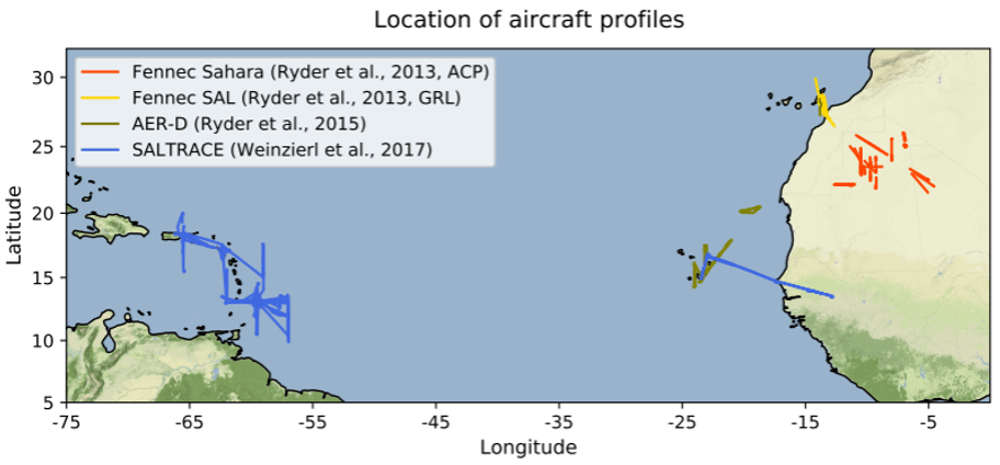
First, we compared in-situ aircraft observations to a climate model simulation to assess the degree to which the model was struggling to represent coarse particle transport from the Sahara across the Atlantic to the Caribbean. Measuring particles up to 300 um in diameter, the Fennec, AER-D and SALTRACE campaigns provide observations at three stages of transport throughout the lifetime of dust in the atmosphere (near emission, moving over the ocean and at distance from the Sahara; Figure 1). Using these observations, we assess a Met Office Unified Model HadGEM3 configuration. This model has six dust size bins, ranging from 0.063-63.2 um diameter. This is a much larger upper bound than most climate models, which tend to have an upper bound at 10-20 um.
We found that the model significantly underestimates the total mass of mineral dust in the atmosphere, as well as the fraction of dust mass made up of coarse particles. This happens at all locations, including at the Sahara: firstly, this suggests that the model is not emitting enough coarse particles to begin with and secondly, the growing model underestimation with distance suggests that the coarse particles are being deposited too quickly. By looking further into the model, we found that the coarsest particles (20-63.2 um) were lost from the atmosphere very quickly, barely surpassing Cape Verde in their westwards transport. Whereas in the observations, these coarsest particles were still present at the Caribbean, representing ~20% of the total dust mass. We also found that the distribution of coarse particles tended to have a stronger dependence on altitude than in the observations, with fewer particles observed at higher altitudes. This work has been written up into a paper which is currently undergoing review, but can be seen in preprint; Ratcliffe et al., (preprint).
Sensitivity Testing of the Model
Now that we have confirmed that the model is struggling to retain coarse particles for long- range transport, we want to work out if any of the model processes involved in transport and deposition could be over- or under-active in coarse particle transport. This involved turning off individual processes one at a time and seeing what impact it has on the dust transport. As we wanted to focus on the impact to coarse particle transport, we needed to start with an improved emission distribution at the Sahara, so we tuned the model to better match the observations from the Fennec campaign.
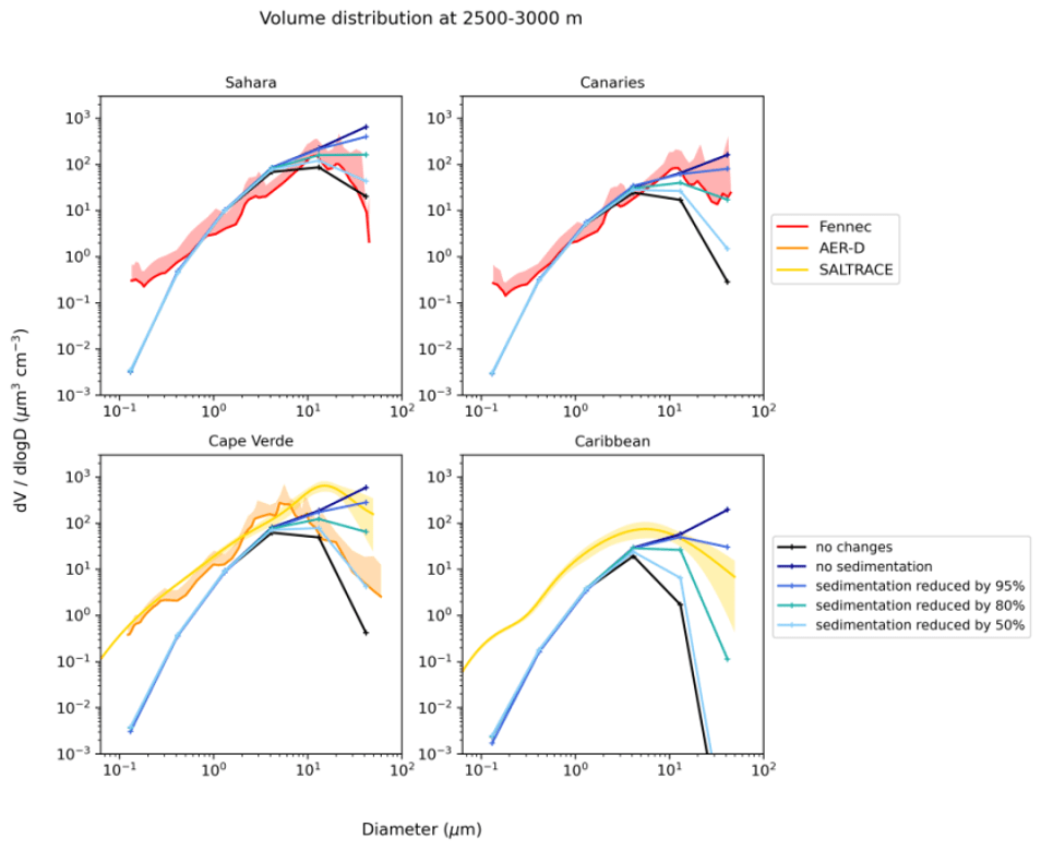
In our first tests we decided to ‘turn off’ or reduce gravitational settling of dust particles in the model to see what happens if we eliminate the greatest removal mechanism for coarse particles. Figure 2 shows the volume size distribution of these gravitational settling model experiments against the observations. We found that completely removing gravitational settling increased the mass of coarse particles too much, while having little to no effect on the fine particles. We found that to bring the model into better agreement with the observations, sedimentation needs to be reduced by ~50% at the Sahara and more than 80% at the Caribbean.
We also tested the sensitivity of turbulent mixing, convective mixing and wet deposition on coarse dust transport; however, these experiments did not have as great of an impact on coarse transport as the sedimentation. We found that removing the mixing mechanisms resulted in decreased vertical transport of dust which tended to reduce the horizontal transport. We also carried out an experiment where we doubled the convective mixing, and this did show improved vertical and horizontal transport. Finally, when we removed wet deposition of dust, we found that it had a greater impact on the fine particles, less so on the coarse particles, suggesting that wet deposition is the main removal mechanism for the four finest size bins in the model.
Final Experiment
Now that we know our coarse particles are settling out too quickly and sit a bit too low in the atmosphere, we come to our final set of experiments. Let’s say that our coarse particles in the model and our dust scheme are actually set up perfectly, then could it be the meteorology in the model which is wrong? If the coarse particles were mixed higher up at the Sahara, then would they reach faster horizontal winds to travel further across the Atlantic? To test this theory, I hacked the files which the model uses to start a simulation, and I put all the dust over the Sahara up to the top of the dusty layer (~5 km). We found this increased the lifetime of the coarsest particles so that it took twice as long to lose 50% of the starting mass. This unfortunately only slightly improved transport distance as the particles were still lost relatively quickly. After checking the vertical winds in the model, we found that they were an order of magnitude smaller at the Sahara, Canaries and Cape Verde than the observations made during the field campaigns. This suggests that if the vertical winds were stronger, they could initially raise the dust higher and keep the coarse particles raised higher for longer, extending their atmospheric lifetime.
Summarised Conclusions
To summarise what I’ve found during my PhD:
- The model underestimates coarse mass at emission and the underestimation is exacerbated with westwards transport.
- Altering the settling velocity of dust in the model brings the model into better agreement with the observations.
- a. Turbulent mixing, convective mixing and wet deposition have minimal impact on coarse transport.
- Lofting the coarse particles higher initially improves transport minimally.
- a. Vertical winds in the model are an order of magnitude too small.
So what’s next?
If we’ve found that the coarse particles are settling out the atmosphere too quickly (by potentially more than 80%), would that suggest that the deposition equations are wrong and are overestimating particle deposition? So, we change those and everything’s fixed, right? I wish. Unfortunately, the deposition equations are one of the things that we are more scientifically sure of, so our results mean that there’s something happening to the coarse particles that we aren’t modelling which is able to counteract their settling velocity by a very significant amount. Our finding that the vertical winds are too small could be a part of this. Other recent research suggests that processes such as particle asphericity, triboelectrification, vertical mixing and turbulent mixing (has been shown to help in a higher-resolution (not climate) model) in the atmosphere could enhance coarse particle transport.
Huneeus, N., Schulz, M., Balkanski, Y., Griesfeller, J., Prospero, J., Kinne, S., Bauer, S., Boucher, O., Chin, M., Dentener, F., Diehl, T., Easter, R., Fillmore, D., Ghan, S., Ginoux, P., Grini, A., Horowitz, L., Koch, D., Krol, M. C., Landing, W., Liu, X., Mahowald, N., Miller, R., Morcrette, J.-J., Myhre, G., Penner, J., Perlwitz, J., Stier, P., Takemura, T., and Zender, C. S. 2011. Global dust model intercomparison in AeroCom phase I. Atmospheric Chemistry and Physics. 11(15), pp. 7781-7816
Kok, J. F., Storelvmo, T., Karydis, V. A., Adebiyi, A. A., Mahowald, N. M., Evan, A. T., He, C., and Leung, D. M. Jan. 2023. Mineral dust aerosol impacts on global climate and climate change. Nature Reviews Earth Environment 2023, pp. 1–16. url: https://www.nature.com/articles/s43017-022-00379-5
RatcliLe, N. G., Ryder, C. L., Bellouin, N., Woodward, S., Jones, A., Johnson, B., Weinzierl, B., Wieland, L.-M., and Gasteiger, J.: Long range transport of coarse mineral dust: an evaluation of the Met Office Unified Model against aircraft observations, EGUsphere [preprint], https://doi.org/10.5194/egusphere-2024-806, 2024
Ryder, C. L., Highwood, E. J., Walser, A., Seibert, P., Philipp, A., and Weinzierl, B. 2019. Coarse and giant particles are ubiquitous in Saharan dust export regions and are radiatively significant over the Sahara. Atmospheric Chemistry and Physics. 19(24), pp. 15353–15376
Shao, Y., Wyrwoll, K.-H., Chappell, A., Huang, J., Lin, Z., McTainsh, G. H., Mikami, M., Tanaka, T. Y., Wang, X., and Yoon, S. 2011. Dust cycle: An emerging core theme in Earth system science. Aeolian Research. 2(4), pp. 181–204
 ) and particulate matter (PM
 ) – particles of about 1/20th of the width of a hair strand – can get into our lungs and cause inflammation, alter their function, or otherwise cause trouble for the cardiovascular system – especially in people with existing underlying respiratory conditions. Although high pollution episodes in the UK are infrequent, the public becomes aware of the associated problems during events such as red skies, in part caused by long-range transport of Saharan dust. Furthermore, the World Health Organisation (WHO) estimates that 85% of UK towns regularly exceed the safe annual PM
 (nitrogen dioxide) using the operational air quality forecasting model in the UK, the Air Quality in the Unified Model (AQUM). This model produces an hourly air quality forecast issued to the public by DEFRA in the form of a Daily Air Quality Index (DAQI) and is verified against surface-based observations from the Automatic Urban and Rural Network (AURN).


 and (right)
  .
. , corresponding to a maximal wavenumber of
  , and
, and  . The former represents the approximate resolution of global NWP models (~ 20 km), and the latter represents a resolution about 1000 times finer so that the shallower mesoscale range is much better resolved. Figure 2 shows the growth of a small-scale, small-amplitude initial error under these model settings.
 , so that the parameters
  and
and  are functions of the wavenumber / scale. Among the parameters, a describes the rate of error growth, the larger the quicker. A dimensional argument suggests that
  , so that
  should be constant for a
  , and should grow
  -fold for every decade of wavenumbers in the case of a
  (1 to 2 km), much smaller in scale than the transition between the
  (300 to 600 km). See Figure 3 for details.
 , for truncations (left)
  and (right)
  .
. . In other words, motions at 1 to 2 km have to be fully resolved in order for error growth in the small scales be correctly represented. This would mean a grid resolution of ~ 250 m after accounting for the need of a dissipation range in a numerical model (Skamarock 2004).


