(Some) Space Weather Forecasts are Less Certain during Solar Minimum than Solar Maximum

Dechen Gyeltschen (d.l.gyeltshen@pgr.reading.ac.uk)

Summary of Gyeltshen, D. L., et al. (2026) 

What is space weather?

Space weather refers to the short-term changes in the space environment of our solar system. We tend to focus on near-Earth space due to its direct impact on human life and infrastructure. Extreme space weather events can cause disruptions to satellite operations, navigation systems, radio communication, power grids, and rail networks. Additionally, they expose humans in space or on high-altitude flights to harmful radiation and energetic particles. Although mitigation procedures are being developed and refined, their efficacy relies on the accuracy of extreme space weather forecasts. As such, understanding causal phenomena such as solar eruptive processes and high-speed solar wind remains a high priority for improving prediction accuracy. 

Coronal Mass Ejections (CMEs) are drivers of the most severe space weather. They consist of a large structure of plasma and an accompanying magnetic field that have a typical Sun-Earth transit time of 1-5 days. This range exists because a) CMEs are ejected at different speeds and b) CMEs interact with the background ‘ambient’ solar wind and can be accelerated/decelerated due to drag forces. Current CME transit time predictions possess errors on the order ± 10 hours.

How are forecasts made?

Identifying sources of these errors requires an understanding of how CME transit time forecasts are made. The forecast process is outlined as follows, with a visual summary provided in Figure 1: 

  • Information about the Sun’s magnetic field structure in the form of magnetograms is used as initial data. 
  • These are fed into coronal models to generate ambient solar wind speed profiles at 0.1 Astronomical Units from the Sun (1 AU ~ 150 million kilometers). 
  • CME parameters are derived from white light coronagraph images and extrapolated to 0.1 AU. 
  • Together they serve as initial conditions for heliospheric models that simulate CME propagation to Earth and other planetary bodies.  
Figure 1: Schematic of standard space weather forecasting method. From top left to bottom right: A magnetogram, a coronagraph, coronal modelling, derivation of CME parameters, heliospheric modelling to Earth and to outer planets (Owens, M. J., et al. (2026)).

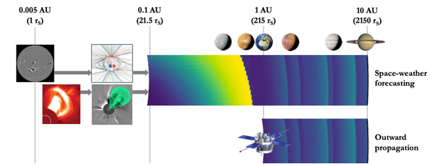
While the models used are imperfect, transit time errors largely stem from initial uncertainties in observations of CME parameters and ambient solar wind conditions.  

What did we do?

Though the sources of transit time errors are identified, the extents of their contributions vary, and isolating individual error contributions for observed events is difficult. In particular, the ambient solar wind properties exhibit substantial variability over the solar cycle. Observations show that during solar minimum, Earth intercepts interchangeable fast and slow winds over the course of a month. On the other hand, the solar wind during solar maximum is less stark in its longitudinal gradients. Does this structural difference between solar cycle phases change the ambient solar wind influence on CME propagation? If yes, by how much?  

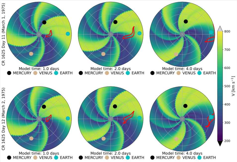
We performed simulations of CME propagation using the Heliospheric Upwind eXtrapolation with time-dependence (HUXt) solar wind model to answer these questions. HUXt approximates the solar wind as a one-dimensional and hydrodynamic flow, which allows for low computational cost. We used realistic solar wind data to simulate a statistically average CME and a fast CME every day between 1975 – 2024 (4.5 solar cycles). This is 18,000 runs and 126,000 simulation days (for each CME)! This gave us a dataset of daily CME transit times to Earth that was later used for the analyses. An example of two such simulations is provided in Figure 2. 

Figure 2: Snapshots of solar wind speed in the solar equatorial plane at three different times (from left to right, shown times are 1, 2, and 4 days after CME launch) from two HUXt simulations. The CME is shown by the red outline. Date labels on the left denote initiation time: the top plots were initialized just 1 day before the lower plots, but the arrival times vary a lot! 

What did we find out?

From the dataset of daily transit times, we calculated the monthly medians and interquartile ranges. We used the median to characterise the typical transit time, and the interquartile range to represent short-term variability of transit time. The distributions for these metrics are shown in Figure 3 for both types of CMEs. 

Figure 3: Top: Distributions of monthly transit time medians, during solar minimum and maximum solar phases for average and fast CMEs. Dotted lines represent median values for the distributions. Bottom: The same for distributions of the monthly interquartile range. 

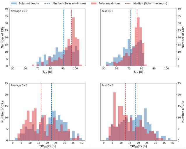
Figure 3 tells us three things: 

  • CMEs arrive faster during solar minimum: the median values show that average CMEs arrive about 5 hours earlier during solar minimum. This is because CMEs encounter either slow or fast wind during solar minimum, but solar maximum presents mostly slow wind that does not accelerate any CME to the same degree. 
  • Transit times are more variable (~6h more variable for an average CME) during solar minimum. The design of our experiment dictates that this effect purely arises from the change in ambient solar wind structure over a solar cycle. 
  • These results are true for both CME types.  

In other words, even identical CMEs can exhibit a range of transit times due to changes in the ambient solar wind structure. Moreover, the magnitude of this variability peaks during solar minimum. It implies that in the absence of accurate ambient solar wind conditions, CME arrivals are intrinsically less predictable during solar minimum than solar maximum. Additionally, the penalty for incorrectly modelling the ambient solar wind—for example, small errors in speed gradients or the position of high-speed streams—is greater during solar minimum. 

Main Takeaways

  • During solar minimum, the arrival time of coronal mass ejections at Earth is roughly twice as uncertain due to the influence of the ambient solar wind compared to solar maximum. 
  • Importance of ambient solar wind representation during solar minimum is emphasised.  

The importance of anticyclonic synoptic eddies for atmospheric block persistence and forecasts

Charlie Suitters – c.c.suitters@pgr.reading.ac.uk

The Beast from the East, the record-breaking winter warmth of February 2020, the Canadian heat dome of 2022…what do these three events have in common? Well, many things I’m sure, but most relevantly for this blog post is that they all coincided with the same phenomenon – atmospheric blocking.

So what exactly is a block? An atmospheric block is a persistent, large-scale, quasi-stationary high-pressure system sometimes found in the mid-latitudes. The prolonged subsidence associated with the high pressure suppresses cloud formation, therefore blocks are often associated with clear, sunny skies, calm winds, and temperature extremes. Their impacts can be diverse, including both extreme heat and extreme cold, drought, poor air quality, and increased energy demand (Kautz et al., 2022). 

Despite the range of hazards that blocking can bring, we still do not fully understand the dynamics that cause a block to start, maintain itself, and decay (Woollings et al., 2018). In reality, many different mechanisms are at play, but the importance of each process can vary between location, season, and individual block events (Miller and Wang, 2022). One process that is known to be important is the interaction between blocks and smaller synoptic-scale transient eddies (Shutts, 1983; Yamazaki and Itoh, 2013). By studying a 43-year climatology of atmospheric blocks and their anticyclonic eddies (both defined by regions of anomalously high 500 hPa geopotential height), I have found that on average, longer blocks absorb more synoptic anticyclones, which “tops up their anticyclonicness” and allows them to persist longer (Fig. 1).

Figure 1: average number of anticyclonic eddies per block for the Euro-Atlantic (left) and North Pacific (right). Block persistence is defined as the quartiles (Q1, Q2, Q3) of all blocks in winter (blue) and summer (red). From Suitters et al. (2023).

It’s great that we now know this relationship, however it would be beneficial to know if these interactions are forecasted well. If they are not, it might explain our shortcomings in predicting the longevity of a block event (Ferranti et al., 2015).  I explore this with a case study from March 2021 using ensemble forecasts from MOGREPS-G. Fortunately, this block in March 2021 was not associated with any severe weather, but it was still not forecasted well. In Figure 2, I show normalised errors in the strength, size, and location of the block, at the time of block onset, for each ensemble member from a range of different initialisation times. In these plots, a negative (positive) value means that the block was forecast to be too weak (strong) or too small (large), and the larger the error in the location, the further away the forecast block was from reality. In general, the onset of this block was forecast to be to be too weak and too small, though there was considerable spread within the ensemble (Fig. 2). Certainty in the forecast was only achieved at relatively small lead times.

Figure 2: Normalised errors in the intensity (left), area (centre), and location of the block’s centre of mass (right), at a validity time of 2021-03-14 12 UTC (the time of onset). Each ensemble member’s error from a particular initialisation time is shown by the grey dots, and the ensemble mean is shown in black. When Z, A, or L are zero, the forecast has a “perfect” replication for this metric of the block (when compared to ERA5 reanalysis).

Now for the interesting bit – what causes the uncertainty in forecasting of the onset this European blocking event? To examine this, I grouped forecast members from an initialisation time of 8 March 2021 according to their ability to replicate the real block: the entire MOGREPS-G mean, members that either have no block or a very small block (Group G), members that perform best (Group H), and members that predict area well, but have the block in the wrong location (Group I). Then, I take the mean geopotential height anomalies () at each time step in each group, and compare these fields between groups to see if I can find a source of forecast error.

This is shown as an animation in Fig. 3. The animation starts at the time of block onset, and goes back in time to selected validity times, as shown at the top of the figure. The domain of the plot also changes in each frame, gradually moving westwards across the Atlantic. By looking at the ERA5 (the “real”) evolution of the block, we see that the onset of the European block was the result of an anticyclonic transient eddy breaking off from an upstream blocking event over North America. However, none of the aforementioned groups of members accurately simulate this vortex shedding from the North American block. In most cases, the eddy leaving the North American block is either too weak or non-existent (as shown by the blue shading, representing that the forecast is much weaker than in ERA5), which resulted in a lack of Eastern Atlantic blocking altogether. Only the group that modelled the block well (Group H) had a sizeable eddy breaking off from the upstream block, but even in this case it was too weak (paler blue shading). Therefore, the uncertain block onset in this case is directly related to the way in which an anticyclonic eddy was forecast to travel (or not) across the Atlantic, from a pre-existing block upstream. This is interesting because the North American block itself was modelled well, yet the eddy that broke off it was not, which was vital for the onset of the Euro-Atlantic block.

To conclude, this is an important finding because it shows the need to accurately model synoptic-scale features in the medium range in order to accurately predict blocking. If these eddies are absent in a forecast, a block might not even form (as I have shown), and therefore potentially hazardous weather conditions would not be forecast until much shorter lead times. My work shows the role of anticyclonic eddies towards the persistence and forecasting of blocks, which until now had not be considered in detail.

References

Kautz, L., Martius, O., Pfahl, S., Pinto, J.G., Ramos, A.M., Sousa, P.M., and Woollings, T., 2022. “Atmospheric blocking and weather extremes over the Euro-Atlantic sector–a review.” Weather and climate dynamics, 3(1), pp305-336.

Miller, D.E. and Wang, Z., 2022. Northern Hemisphere winter blocking: differing onset mechanisms across regions. Journal of the Atmospheric Sciences, 79(5), pp.1291-1309.

Shutts, G.J., 1983. The propagation of eddies in diffluent jetstreams: Eddy vorticity forcing of ‘blocking’ flow fields. Quarterly Journal of the Royal Meteorological Society, 109(462), pp.737-761.

Suitters, C.C., Martínez-Alvarado, O., Hodges, K.I., Schiemann, R.K. and Ackerley, D., 2023. Transient anticyclonic eddies and their relationship to atmospheric block persistence. Weather and Climate Dynamics, 4(3), pp.683-700.

Woollings, T., Barriopedro, D., Methven, J., Son, S.W., Martius, O., Harvey, B., Sillmann, J., Lupo, A.R. and Seneviratne, S., 2018. Blocking and its response to climate change. Current climate change reports, 4, pp.287-300.

Yamazaki, A. and Itoh, H., 2013. Vortex–vortex interactions for the maintenance of blocking. Part I: The selective absorption mechanism and a case study. Journal of the Atmospheric Sciences, 70(3), pp.725-742.

New Forecast Model Provides First Global Scale Seasonal River Flow Forecasts

new_web_figure2_rivernetwork

Over the past ~decade, extended-range forecasts of river flow have begun to emerge around the globe, combining meteorological forecasts with hydrological models to provide seasonal hydro-meteorological outlooks. Seasonal forecasts of river flow could be useful in providing early indications of potential floods and droughts; information that could be of benefit for disaster risk reduction, resilience and humanitarian aid, alongside applications in agriculture and water resource management.

While seasonal river flow forecasting systems exist for some regions around the world, such as the U.S., Australia, Africa and Europe, the forecasts are not always accessible, and forecasts in other regions and at the global scale are few and far between.  In order to gain a global overview of the upcoming hydrological situation, other information tends to be used – for example historical probabilities based on past conditions, or seasonal forecasts of precipitation. However, precipitation forecasts may not be the best indicator of floodiness, as the link between precipitation and floodiness is non-linear. A recent paper by Coughlan-de-Perez et al (2017), “should seasonal rainfall forecasts be used for flood preparedness?”, states:

“Ultimately, the most informative forecasts of flood hazard at the seasonal scale are streamflow forecasts using hydrological models calibrated for individual river basins. While this is more computationally and resource intensive, better forecasts of seasonal flood risk could be of immense use to the disaster preparedness community.”

twitter_screenshotOver the past months, researchers in the Water@Reading* research group have been working with the European Centre for Medium-Range Weather Forecasts (ECMWF), to set up a new global scale hydro-meteorological seasonal forecasting system. Last week, on 10th November 2017, the new forecasting system was officially launched as an addition to the Global Flood Awareness System (GloFAS). GloFAS is co-developed by ECMWF and the European Commission’s Joint Research Centre (JRC), as part of the Copernicus Emergency Management Services, and provides flood forecasts for the entire globe up to 30 days in advance. Now, GloFAS also provides seasonal river flow outlooks for the global river network, out to 4 months ahead – meaning that for the first time, operational seasonal river flow forecasts exist at the global scale – providing globally consistent forecasts, and forecasts for countries and regions where no other forecasts are available.

The new seasonal outlook is produced by forcing the Lisflood hydrological river routing model with surface and sub-surface runoff from SEAS5, the latest version of ECMWF’s seasonal forecasting system, (also launched last week), which consists of 51 ensemble members at ~35km horizontal resolution. Lisflood simulates the groundwater and routing processes, producing a probabilistic forecast of river flow at 0.1o horizontal resolution (~10km, the resolution of Lisflood) out to four months, initialised using the latest ERA-5 model reanalysis.

The seasonal outlook is displayed as three new layers in the GloFAS web interface, which is publicly (and freely) available at www.globalfloods.eu. The first of these gives a global overview of the maximum probability of unusually high or low river flow (defined as flow exceeding the 80th or falling below the 20th percentile of the model climatology), during the 4-month forecast horizon, in each of the 306 major world river basins used in GloFAS-Seasonal.

new_web_figure1_basins
The new GloFAS Seasonal Outlook Basin Overview and River Network Layers.

The second layer provides further sub-basin-scale detail, by displaying the global river network (all pixels with an upstream area >1500km2), again coloured according to the maximum probability of unusually high or low river flow during the 4-month forecast horizon. In the third layer, reporting points with global coverage are displayed, where more forecast information is available. At these points, an ensemble hydrograph is provided showing the 4-month forecast of river flow, with thresholds for comparison of the forecast to typical or extreme conditions based on the model climatology. Also displayed is a persistence diagram showing the weekly probability of exceedance for the current and previous three forecasts.

blog_screenshot
The new GloFAS Seasonal Outlook showing the river network and reporting points providing hydrographs and persistence diagrams.

Over the coming months, an evaluation of the system will be completed – for now, users are advised to evaluate the forecasts for their particular application. We welcome any feedback on the forecast visualisations and skill – feel free to contact me at the email address below!

To find out more, you can see the University’s press release here, further information on SEAS5 here, and the user information on the seasonal outlook GloFAS layers here.

*Water@Reading is “a vibrant cross-faculty centre of research excellence at the University of Reading, delivering world class knowledge in water science, policy and societal impacts for the UK and internationally.”

Full list of collaborators: 

Rebecca Emerton1,2, Ervin Zsoter1,2, Louise Arnal1,2, Prof. Hannah Cloke1, Dr. Liz Stephens1, Dr. Florian Pappenberger2, Prof. Christel Prudhomme2, Dr Peter Salamon3, Davide Muraro3, Gabriele Mantovani3

1 University of Reading
2 ECMWF
3 European Commission JRC

Contact: r.e.emerton@pgr.reading.ac.uk