Space weather refers to the short-term changes in the space environment of our solar system. We tend to focus on near-Earth space due to its direct impact on human life and infrastructure. Extreme space weather events can cause disruptions to satellite operations, navigation systems, radio communication, power grids, and rail networks. Additionally, they expose humans in space or on high-altitude flights to harmful radiation and energetic particles. Although mitigation procedures are being developed and refined, their efficacy relies on the accuracy of extreme space weather forecasts. As such, understanding causal phenomena such as solar eruptive processes and high-speed solar wind remains a high priority for improving prediction accuracy.
Coronal Mass Ejections (CMEs) are drivers of the most severe space weather. They consist of a large structure of plasma and an accompanying magnetic field that have a typical Sun-Earth transit time of 1-5 days. This range exists because a) CMEs are ejected at different speeds and b) CMEs interact with the background ‘ambient’ solar wind and can be accelerated/decelerated due to drag forces. Current CME transit time predictions possess errors on the order ± 10 hours.
How are forecasts made?
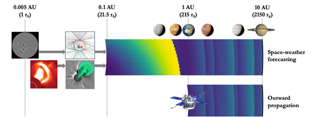
Identifying sources of these errors requires an understanding of how CME transit time forecasts are made. The forecast process is outlined as follows, with a visual summary provided in Figure 1:
Information about the Sun’s magnetic field structure in the form of magnetograms is used as initial data.
These are fed into coronal models to generate ambient solar wind speed profiles at 0.1 Astronomical Units from the Sun (1 AU ~ 150 million kilometers).
CME parameters are derived from white light coronagraph images and extrapolated to 0.1 AU.
Together they serve as initial conditions for heliospheric models that simulate CME propagation to Earth and other planetary bodies.
Figure 1: Schematic of standard space weather forecasting method. From top left to bottom right: A magnetogram, a coronagraph, coronal modelling, derivation of CME parameters, heliospheric modelling to Earth and to outer planets (Owens, M. J., et al. (2026)).
While the models used are imperfect, transit time errors largely stem from initial uncertainties in observations of CME parameters and ambient solar wind conditions.
What did we do?
Though the sources of transit time errors are identified, the extents of their contributions vary, and isolating individual error contributions for observed events is difficult. In particular, the ambient solar wind properties exhibit substantial variability over the solar cycle. Observations show that during solar minimum, Earth intercepts interchangeable fast and slow winds over the course of a month. On the other hand, the solar wind during solar maximum is less stark in its longitudinal gradients. Does this structural difference between solar cycle phases change the ambient solar wind influence on CME propagation? If yes, by how much?
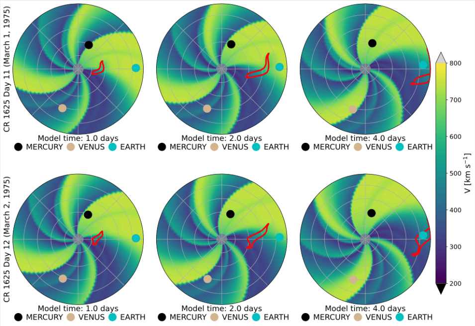
We performed simulations of CME propagation using the Heliospheric Upwind eXtrapolation with time-dependence (HUXt) solar wind model to answer these questions. HUXt approximates the solar wind as a one-dimensional and hydrodynamic flow, which allows for low computational cost. We used realistic solar wind data to simulate a statistically average CME and a fast CME every day between 1975 – 2024 (4.5 solar cycles). This is 18,000 runs and 126,000 simulation days (for each CME)! This gave us a dataset of daily CME transit times to Earth that was later used for the analyses. An example of two such simulations is provided in Figure 2.
Figure 2: Snapshots of solar wind speed in the solar equatorial plane at three different times (from left to right, shown times are 1, 2, and 4 days after CME launch) from two HUXt simulations. The CME is shown by the red outline. Date labels on the left denote initiation time: the top plots were initialized just 1 day before the lower plots, but the arrival times vary a lot!
What did we find out?
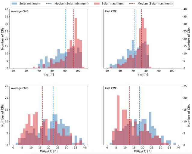
From the dataset of daily transit times, we calculated the monthly medians and interquartile ranges. We used the median to characterise the typical transit time, and the interquartile range to represent short-term variability of transit time. The distributions for these metrics are shown in Figure 3 for both types of CMEs.
Figure 3: Top: Distributions of monthly transit time medians, during solar minimum and maximum solar phases for average and fast CMEs. Dotted lines represent median values for the distributions. Bottom: The same for distributions of the monthly interquartile range.
Figure 3 tells us three things:
CMEs arrive faster during solar minimum: the median values show that average CMEs arrive about 5 hours earlier during solar minimum. This is because CMEs encounter either slow or fast wind during solar minimum, but solar maximum presents mostly slow wind that does not accelerate any CME to the same degree.
Transit times are more variable (~6h more variable for an average CME) during solar minimum. The design of our experiment dictates that this effect purely arises from the change in ambient solar wind structure over a solar cycle.
These results are true for both CME types.
In other words, even identical CMEs can exhibit a range of transit times due to changes in the ambient solar wind structure. Moreover, the magnitude of this variability peaks during solar minimum. It implies that in the absence of accurate ambient solar wind conditions, CME arrivals are intrinsically less predictable during solar minimum than solar maximum. Additionally, the penalty for incorrectly modelling the ambient solar wind—for example, small errors in speed gradients or the position of high-speed streams—is greater during solar minimum.
Main Takeaways
During solar minimum, the arrival time of coronal mass ejections at Earth is roughly twice as uncertain due to the influence of the ambient solar wind compared to solar maximum.
Importance of ambient solar wind representation during solar minimum is emphasised.
By Douglas Mulangwa – d.mulangwa@pgr.reading.ac.uk
Between 2019 and 2024, East Africa experienced one of the most persistent high-water periods in modern history: a flood that simply would not recede. Lakes Victoria, Kyoga, and Albert all rose to exceptional levels, and the Sudd Wetland in South Sudan expanded to an unprecedented 163,000 square kilometres in 2022. More than two million people were affected across Uganda and South Sudan as settlements, roads, and farmland remained inundated for months.
At first, 2022 puzzled stakeholders, observers and scientists alike. Rainfall across much of the region was below average that year, yet flooding in the Sudd intensified. This prompted a closer look at the wider hydrological system. Conventional explanations based on local rainfall failed to account for why the water would not recede. The answer, it turned out, lay far upstream and more than a year earlier, hidden within the White Nile’s connected lakes and wetlands.
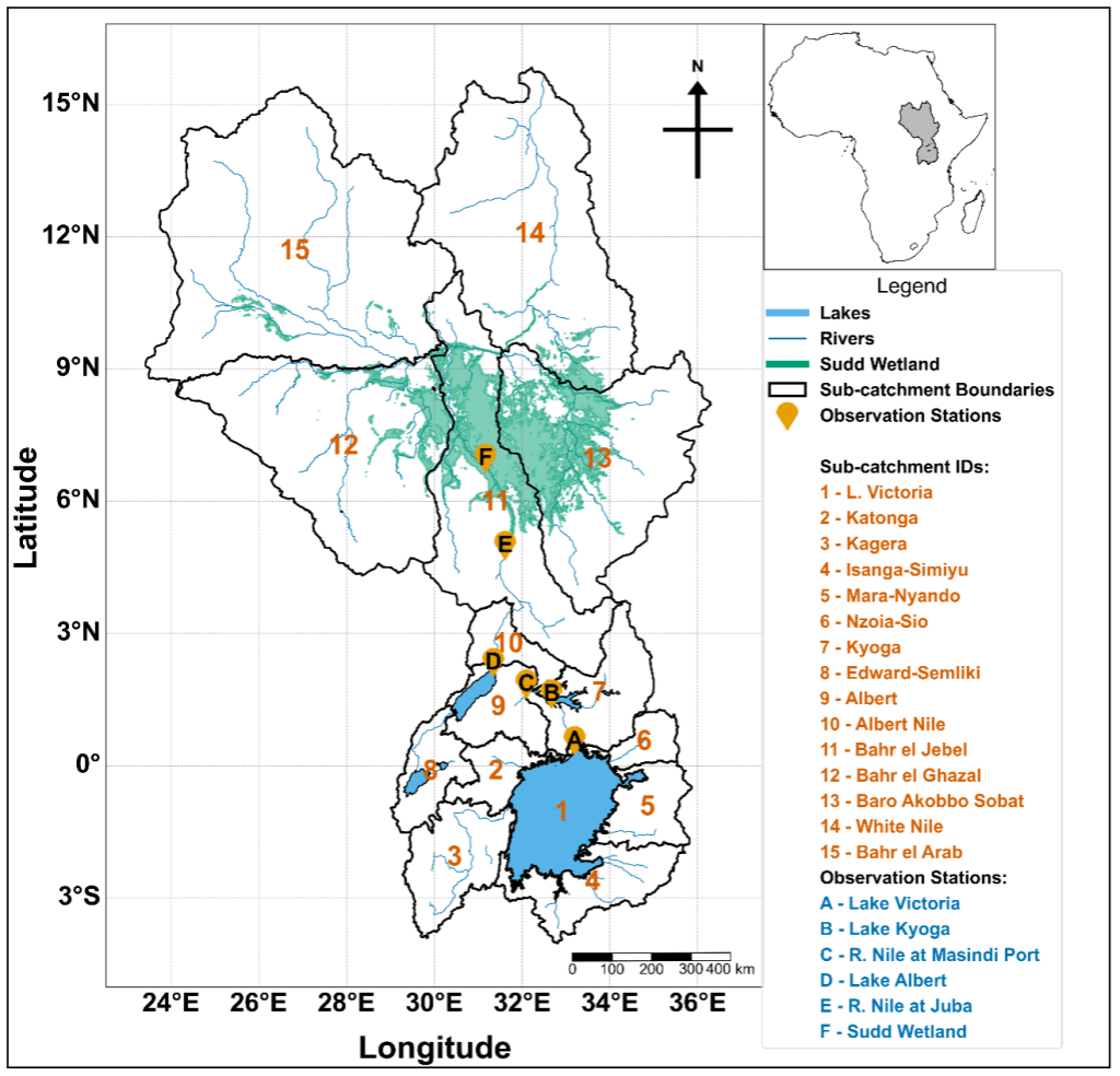
Figure 1: Map of the White Nile Basin showing delineated sub-catchments, lakes, major rivers, and the Sudd Wetland extent. Sub-catchments are labelled numerically (1–15) with names listed in the legend. Observation stations (A–F) mark key hydrological data collection locations used in this study: Lake Victoria (A), Lake Kyoga (B), River Nile at Masindi Port (C), Lake Albert (D), River Nile at Juba (E), and the Sudd Wetland (F). Background river networks and sub-catchment boundaries are derived from the HydroSHED dataset, and wetland extent is based on MODIS flood mask composites. The map is projected in geographic coordinates (EPSG:4326) with a graduated scale bar for accurate distance representation using UTM Zone 36N.
The White Nile: A Basin with Memory
The White Nile forms one of the world’s most complex lake, river, and wetland systems, extending from Lake Victoria through Lakes Kyoga and Albert into the Sudd. Hydrologically, it is a system of connected reservoirs that store, delay, and gradually release floodwaters downstream.
For decades, operational planning assumed that floodwaters take roughly five months to travel from Lake Victoria to the Sudd. That estimate was never actually tested with data; it originated as a rule of thumb based on Lake Victoria annual maxima in May and peak flooding in South Sudan in September/October.
Our recent study challenged that assumption. By combining daily lake-level and discharge data (1950–2024) with CHIRPS rainfall and MODIS flood-extent records (2002–2024), we tracked how flood peaks propagated through the system, segment by segment. Using an automated peak-matching algorithm, we quantified the lag between successive annual maxima peaks in Lake Victoria, Lake Kyoga, Lake Albert, and the Sudd Wetland.
The unprecedented high-water regime of 2019-2024
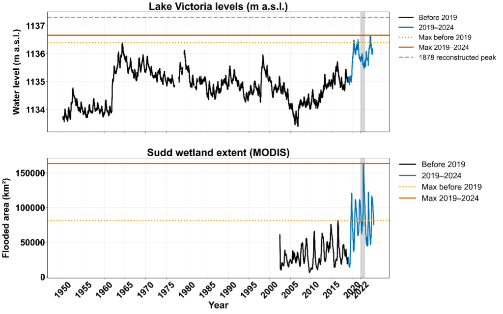
Figure 2: Lake Victoria water levels (1950–2024) and Sudd Wetland extents (2002–2024), with the 2019–2024 anomalous period shown in dark blue and earlier observations in black. The orange dotted line marks the pre-2019 maximum, while the solid vermillion line denotes the highest peak observed during 2019–2024. The dashed magenta line represents the reconstructed 1878 Lake Victoria peak (1137.3 m a.s.l.) from Nicholson & Yin (2001). The shaded grey band highlights the 2022 flood year, when the Sudd reached its largest extent in the MODIS record.
Between 2019 and 2024, both Lake Victoria and the Sudd reached record levels. Lake Victoria exceeded its historic 1964 peak in 2020, 2021, and 2024, while the Sudd expanded to more than twice its previous maximum extent. Each year from 2019 to 2024 stayed above any pre-2019 record, revealing that this was not a single flood season but a sustained multi-year regime.
The persistence of the 2019–2024 high-water regime mirrors earlier basin-wide episodes, including the 1961–64 and 1870s floods, when elevated lake levels and wetland extents were sustained across multiple years rather than confined to a single rainy season. However, the 2020s stand out as the most extensive amongst all the episodes since the start of the 20th century. These data confirm that both the headwaters and terminal floodplain remained at record levels for several consecutive years during 2019–2024, highlighting the unprecedented nature of this sustained high-water phase in the modern observational era.
2019–2024: How Multi-Year Rainfall Triggers Propagated a Basin-Wide Flood
The sequence of flood events began with the exceptionally strong positive Indian Ocean Dipole of 2019, which brought extreme rainfall across the Lake Victoria basin. This marked the first in a series of four consecutive anomalous rainfall seasons that sustained elevated inflows into the lake system. The October–December 2019 short rains were among the wettest on record, followed by above-normal rainfall in the March–May 2020 long rains, another wet short-rains season in late 2020, and continued high rainfall through early 2021. Together, these back-to-back wet seasons kept catchments saturated and prevented any significant drawdown of lake levels between seasons. Lake Victoria rose by more than 1.4 metres between September 2019 and May 2020, the highest increase since the 1960s, and remained near the 1960s historical maximum for consecutive years. As that excess water propagated downstream, Lakes Kyoga and Albert filled and stayed high through 2021. Even when regional rainfall weakened in 2022, these upstream lakes continued releasing stored water into the White Nile. The flood peak that reached the Sudd in 2022 corresponded closely to the 2021 Lake Victoria high-water phase.
This sequence shows that the 2022 disaster was not driven by a single rainfall event but by cumulative wetness over multiple seasons. Each lake acted as a slow reservoir that buffered and then released the 2019 to 2021 excess water, resulting in multi-year flooding that persisted long after rainfall had returned to near-normal levels.
Transit Time and Floodwave Propagation
Quantitative tracking showed that it takes an average of 16.8 months for a floodwave to travel from Lake Victoria to the Sudd. The fastest transmission occurs between Victoria and Kyoga (around 4 months), while the slowest and most attenuated segment lies between Albert and the Sudd (around 9 months).
This overturns the long-held assumption of a five-month travel time and reveals a system dominated by floodplain storage and delayed release. The 2019–2021 period showed relatively faster propagation because of high upstream storage, while 2022 exhibited the longest lag as the Sudd absorbed and held vast volumes of water. By establishing this timing empirically, the study offers a more realistic foundation for early-warning systems.
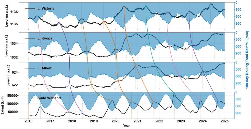
Figure 3: Lake Victoria, Lake Kyoga, and Lake Albert water levels, and Sudd Wetland inundated extent, from 2016 to 2024. Coloured spline curves indicate annual flood-wave trajectories traced from the timing of Lake Victoria annual maxima through the downstream of the White Nile system. Blue shading on the secondary (right) axis shows 180-day rolling rainfall totals over each basin. The panel sequence (Victoria–Kyoga, Kyoga–Albert, Albert–Sudd) highlights the progressive translation of flood waves through the connected lake–river–wetland network.
Wetland Activation and Flood Persistence
Satellite flood-extent maps reveal how the Sudd responded once the inflow arrived. The wetland expanded through multiple activation arms that progressively connected different sub-catchments:
2019: rainfall-fed expansion on the east (Baro–Akobo–Sobat and White Nile sub-basins)
2020–2021: a central-western arm from Bahr el Jebel extending into Bahr el Ghazal and a north-western connection from Bahr el Jebel to Bahr el Arab connected around Bentiu in Unity State.
2022: The two activated arms persisted so the JJAS seasonal rainfall in South Sudan and the inflow from the upstream lakes just compounded the activation leading to the massive flooding in Bentiu, turning the town into an island surrounded by water.
This geometry confirms that the Sudd functions not as a single floodplain but as a network of hydraulically linked basins. Once activated, these wetlands store and recycle water through backwater effects, evaporation, and lateral flow between channels. That internal connectivity explains why flooding persisted long after rainfall declined.
The Bigger Picture
Understanding these long lags is vital for effective flood forecasting and anticipatory humanitarian action. Current early-warning systems in South Sudan and Uganda mainly rely on short-term rainfall forecasts, which cannot capture the multi-season cumulative storage and delayed release that drive multi-year flooding.
By the time floodwaters reach the Sudd Wetland, the hydrological signature of releases from Lake Victoria has been substantially transformed by storage, delay, and attenuation within the intermediate lakes and wetlands. This means that downstream flood conditions are not a direct reflection of upstream releases but the result of cumulative interactions across the basin’s interconnected reservoirs.
The results suggest that antecedent storage conditions in Lakes Victoria, Kyoga, and Albert should be incorporated into regional flood outlooks. When upstream lake levels are exceptionally high, downstream alerts should remain elevated even if rainfall forecasts appear moderate. This approach aligns with impact-based forecasting, where decisions are informed not only by rainfall predictions but also by hydrological memory, system connectivity and potential impact of the floods.
The 2019–2024 high-water regime joins earlier basin-wide flood episodes in the 1870s, 1910s, and 1960s, each linked to multi-year wet phases across the equatorial lakes. The 1961–64 event raised Lake Victoria by about 2.5 metres and reshaped the Nile’s flow for several years. The 1870s flood appears even more extensive, showing that compound, persistent flooding is part of the White Nile’s natural variability.
Climate-change attribution studies indicate that the 2019–2020 rainfall anomaly was intensified by anthropogenic warming, increasing both its magnitude and probability. If such events become more frequent, the basin’s long-memory behaviour could convert short bursts of rainfall into multi-year high-water regimes.
This work reframes how we view the White Nile. It is not a fast, responsive river system but a slow-moving memory corridor in which floodwaves propagate, store, and echo over many months. Recognising this behaviour opens practical opportunities: it enables longer forecast lead times based on upstream indicators, supports coordinated management of lake releases, and strengthens early-action planning for humanitarian agencies across the basin.
It also highlights the need for continued monitoring and data sharing across national borders. Sparse observations remain a major limitation: station gaps, satellite blind spots, and non-public lake-release data all reduce our ability to model the system in real time. Improving this observational backbone is essential if we are to translate scientific insight into effective flood preparedness.
By Douglas Mulangwa (PhD researcher, Department of Meteorology, University of Reading), with contributions from Evet Naturinda, Charles Koboji, Benon T. Zaake, Emily Black, Hannah Cloke, and Elisabeth M. Stephens.
Acknowledgements
This research was conducted under the INFLOW project, funded through the CLARE programme (FCDO and IDRC), with collaboration from the Uganda Ministry of Water and Environment, the South Sudan Ministry of Water Resources and Irrigation, the World Food Programme(WFP), IGAD Climate Prediction and Application Centre (ICPAC), Médecins Sans Frontières (MSF), the Red Cross Red Crescent Climate Centre, Uganda Red Cross Society (URCS), the South Sudan Red Cross Red Crescent Society (SSRCS) and the Red Cross Red Crescent Climate Centre (RCCC).
Convective self-aggregation is the process by which initially randomly scattered convection becomes spontaneously clustered in space despite uniform initial conditions. This process was first identified in numerical models, however it is relevant to real world convection (Holloway et al., 2017). Tropical weather is dominated by convection, and the degree of convective aggregation has important consequences for weather and climate. A more organised regime is associated with reduced cloudiness, increased longwave emission to space (Bretherton et al., 2005), and a higher frequency of long-lasting extreme precipitation events (Bao and Sherwood, 2019).
Because of its relevance to weather and climate, self-aggregation has been the focus of many recent studies. However, there is still much debate as to the processes that cause aggregation. There is great variability in the rate and degree of aggregation between models, and there remains uncertainty as to how aggregation is affected by climate change (Wing et al., 2020). Previous studies have shown that feedbacks between convection and shortwave & longwave radiation are key drivers and maintainers of aggregation (e.g. Wing & Cronin 2016), and that interactive radiation in models is essential for aggregation to occur (Muller & Bony 2015).
This blog summarises results from the first paper from my PhD (Pope et al., 2021), where we develop and use a framework to analyse how radiative interactions with different cloud types contribute to aggregation. We analyse self-aggregation within a set of three idealised simulations of the UK Met Office Unified Model (UM). The simulations are configured in radiative-convective equilibrium over three fixed sea surface temperatures (SSTs) of 295, 300 and 305 K. They are convection permitting models that are 432 × 6048 km2 in size with a 3 km horizontal grid spacing. The simulations neglect the earth’s rotation, so they approximately represent convection over tropical oceans within a warming climate.
Our analysis framework is based on that used in Wing and Emanuel (2014) which uses the variance of vertically-integrated frozen moist static energy (FMSE) as a measure of aggregation. FMSE is a measure of the total energy an air parcel has if all the water (vapour and frozen) was converted to liquid, neglecting its velocity. Variations in vertically-integrated FMSE come from perturbations in temperature and humidity. As aggregation increases, moist regions get moister and dry regions get drier, so the variance of vertically-integrated FMSE increases.
The problem with using FMSE variance as an aggregation metric is that it is highly sensitive to SST. A warmer atmosphere can hold more water vapour via the Clausius-Clapeyron relationship. This means there is a greater difference in FMSE between the moist and dry regions for higher-SST simulations, so the variance of FMSE is typically much greater for higher SSTs. To account for this problem, we normalise FMSE between hypothetical upper and lower limits which are functions of SST. This gives a value of normalised FMSE between 0 and 1.
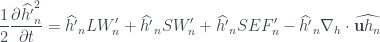
Wing and Emanuel (2014) derive a budget equation for the rate of change of FMSE variance which shows how different processes contribute to aggregation. By rederiving their equation for normalised FMSE , we get:
where is vertically-integrated FMSE, and are the net atmospheric column longwave and shortwave heating rates, is the surface enthalpy flux, made up of the surface latent and sensible heat fluxes, and is the horizontal divergence of the flux. Primes () indicate local anomalies from the instantaneous domain mean. The subscript () denotes a normalised variable which is the original variable divided by the difference between the hypothetical upper and lower limits of . The equation shows that the rate of change of variance (left hand side term) is driven by interactions between anomalies and anomalies in normalised net longwave heating, shortwave heating, surface fluxes and advection.
Figure 1: Hovmöller plots of normalised FMSE for each SST
Figure 2: (a) Time series of vertically-integrated FMSE variance, (b) Time series of normalised vertically-integrated FMSE variance for each SST
We use the variance of as our aggregation metric. Hovmöller plots of are shown in Figure 1 for each of our SSTs. In these plots, is averaged along the short axis of our domains. The plots show how initially randomly-distributed convection organises into bands which expand until the point where there are 4 to 5 quasi-stationary bands of moist convective regions separated by dry subsiding regions. This demonstrates that once our domains become fully-aggregated, the degree of aggregation appears similar. Figure 2a shows time series of each of the variance of , and shows that the variance of non-normalised is ~4 times greater for our 305 K simulations compared to our 295 K simulation. Figure 2b shows time series of the variance of . From this, we can see the convection aggregates faster as SST increases, yet the degree of aggregation remains similar via this metric once the convection is fully aggregated. Values of variance around 10-4 or lower correspond to randomly scattered convection, whereas values greater that 10-3 are associated with strongly aggregated convection.
Figure 3: Maps of (a) cloud condensed water path, (b) vertically-integrated FMSE anomaly, (c) longwave heating anomaly, (d) shortwave heating anomaly. Snapshots at day 100 of the 300 K simulation.
To understand the processes contributing to aggregation, we have to look to Equation 1. We mainly focus on the two radiative terms on the right hand side. The terms show that regions in which the radiative anomalies and the anomalies have the same sign contribute to aggregation. We can start to get an intuitive understanding of this concept by looking at maps of these variables. Figure 3b-d show maps of , and . We can see and are closely correlated since is mainly determined by the shortwave absorption by water vapour. Clouds have little effect on the shortwave heating rates, with ~90% of the shortwave heating rate in cloudy regions being due to absorption by water vapour. is closely linked to cloud condensed water path (Figure 3a). This is because the majority of our clouds are high-topped clouds which, due to their cold cloud tops, are able to prevent longwave radiation escaping to space, so they are associated with positive longwave heating anomalies.
The sensitivity of the budget terms to both aggregation and SST can be seen in Figure 4. This figure is made by creating 50 bins of variance and then averaging the budget terms in space and time for each bin and for each SST. Where the terms are positive, they are helping to increase aggregation. Where they are negative, the terms are opposing aggregation. The terms tend to increase in magnitude since every term has as a factor, which increases with aggregation by definition.
Figure 4: Terms in Equation 1 vs normalised FMSE variance for each SST
In general, we find the longwave term is the dominant driver of aggregation, being insensitive to SST during the growth phase of aggregation. Once the aggregation is mature, the longwave term remains the dominant maintainer of aggregation, however its contribution to aggregation maintenance decreases with SST. The shortwave term is initially small at early times but becomes a key maintainer of aggregation within highly-aggregated environments. This is because humidity variations are initially small, so there is little variation in shortwave heating. Once the convection is aggregated, moist regions are very moist and dry regions are very dry, so there is a large difference in shortwave heating between moist and dry regions. The variations in shortwave heating remain very similar with SST, meaning shortwave heating anomalies contribute the same amount to non-normalised variance. Therefore, shortwave heating contributes less to aggregation at higher SSTs because they contribute to a smaller fraction of anomalies. The radiative terms are balanced by the surface flux term (negative because there is greater evaporation in dry regions) and the advection term (negative because circulations tend to smooth out gradients). The decrease in the magnitude of the radiative terms with SST is balanced by the surface flux and advection terms becoming more positive with SST.
To understand the behaviour of the longwave term, we define different cloud types based on the vertical profile of cloud, assigning one cloud type per grid box in a similar way to Hill et al. (2018). We define a lower and upper level pressure threshold, assigning cloud below the lower threshold to a “Low” category, cloud above the upper threshold to a “High” category, and cloud in between to a “Mid” category. If cloud occurs in more than one of these layers, then it is assigned to a combined category. In total, there are eight cloud types: Clear, Low, Mid, Mid & Low, High, High & Low, High & Mid, and Deep. We can then find each cloud type’s contribution to the longwave term by multiplying the cloud’s mean [Equation] covariance by its domain fraction.
To see how the cloud type contributions change with aggregation, we define a Growth phase and Mature phase of aggregation. The Growth phase has variance between and and the Mature phase has variance between and . The contribution of longwave interactions with each cloud type to aggregation during these two phases is shown in Figure 5a, with their mean covariance and fraction shown in Figures 5b & c.
Figure 5: Mean (a) contribution to the longwave term in Equation 1, (b) normalised longwave-FMSE covariance, (c) cloud fraction for the Growth phase (dots) and Mature phase (open circles). Data points for each category are in order of SST increasing to the right.
We find that longwave interactions with high-topped clouds and clear regions drive aggregation during the Growth phase (Figure 5a). This is because high clouds are abundant, have positive longwave heating anomalies and occur in moist, high environments. The clear regions are the most abundant category, have typically negative longwave heating anomalies and tend to occur in low regions, so their covariance is positive. During the Growth phase, there is little SST sensitivity within each category. During the Mature phase, longwave interactions with high-topped cloud remain the main maintainer of aggregation however their contribution decreases with SST. This sensitivity is mainly because there is a greater decrease in high-topped cloud fraction with aggregation as SST increases. This also has consequences for the covariance of the clear regions. As high-topped cloud fraction reduces, the domain-mean longwave cooling increases. This makes the radiative cooling of the clear regions less anomalous, resulting in an increasingly negative covariance during the Mature phase as SST increases.
There is great variability in the degrees of aggregation within numerical models, which has important consequences for weather and climate modelling (Wing et al. 2020). With cloud-radiation interactions being crucial for aggregation, understanding how these interactions vary between models may help to explain the differences in aggregation. This study provides a framework by which a comparison of cloud-radiation interactions and their contributions to convective self-aggregation between models and SSTs can be achieved.
Page Break
REFERENCES
Bao, J., & Sherwood, S. C. (2019). The role of convective self-aggregation in extreme instantaneous versus daily precipitation. Journal of Advances in Modeling Earth Systems, 11(1), 19– 33. https://doi.org/10.1029/2018MS001503
Bretherton, C. S., Blossey, P. N., & Khairoutdinov, M. (2005). An energy-balance analysis of deep convective self-aggregation above uniform SST. Journal of the Atmospheric Sciences, 62(12), 4273– 4292. https://doi.org/10.1175/JAS3614.1
Hill, P. G., Allan, R. P., Chiu, J. C., Bodas-Salcedo, A., & Knippertz, P. (2018). Quantifying the contribution of different cloud types to the radiation budget in Southern West Africa. Journal of Climate, 31(13), 5273– 5291. https://doi.org/10.1175/JCLI-D-17-0586.1
Holloway, C. E., Wing, A. A., Bony, S., Muller, C., Masunaga, H., L’Ecuyer, T. S., & Zuidema, P. (2017). Observing convective aggregation. Surveys in Geophysics, 38(6), 1199– 1236. https://doi.org/10.1007/s10712-017-9419-1
Muller, C., & Bony, S. (2015). What favors convective aggregation and why? Geophysical Research Letters, 42(13), 5626– 5634. https://doi.org/10.1002/2015GL064260
Pope, K. N., Holloway, C. E., Jones, T. R., & Stein, T. H. M. (2021). Cloud-radiation interactions and their contributions to convective self-aggregation. Journal of Advances in Modeling Earth Systems, 13, e2021MS002535. https://doi.org/10.1029/2021MS002535
Wing, A. A., & Cronin, T. W. (2016). Self-aggregation of convection in long channel geometry. Quarterly Journal of the Royal Meteorological Society, 142(694), 1– 15. https://doi.org/10.1002/qj.2628
Wing, A. A., & Emanuel, K. A. (2014). Physical mechanisms controlling self-aggregation of convection in idealized numerical modeling simulations. Journal of Advances in Modeling Earth Systems, 6(1), 59– 74. https://doi.org/10.1002/2013MS000269
Wing, A. A., Stauffer, C. L., Becker, T., Reed, K. A., Ahn, M.-S., Arnold, N., & Silvers, L. (2020). Clouds and convective self-aggregation in a multi-model ensemble of radiative-convective equilibrium simulations. Journal of Advances in Modeling Earth Systems, 12(9), e2020MS0021380. https://doi.org/10.1029/2020MS0021380
For my PhD, I research heatwaves and heat stress, with a focus on the African continent. Here I show what the main challenges are for communicating heatwave impacts inspired by a presentation given by Roop Singh of the Red Cross Climate Center at Understanding Risk Forum 2020.
There is no universal definition of heatwaves
Having no agreed definition of a heatwave (also known as extreme heat events) is a huge challenge in communicating risk. However, there is a guideline definition by the World Meteorological Organisation and for the UK an agreed definition as of 2019. In simple terms a heatwave is:
“A period of above average temperatures of 3 or more days in a region’s warm season (i.e. all year in the tropics and in the summer season elsewhere)”
We then have heat stress which is an impact of heatwaves, and is the killer aspect of heat. Heat stress is:
“Build-up of body heat as a result of exertion or external environment”(McGregor, 2018)
Attention Deficit
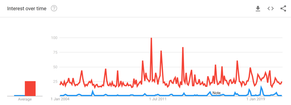
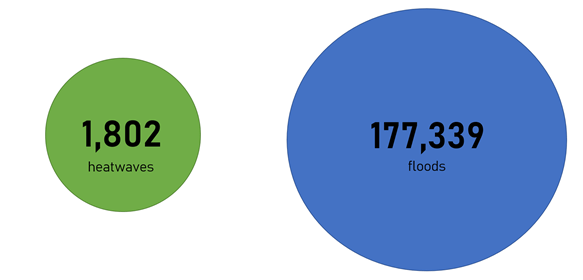
Heatwaves receive low attention in comparison to other natural hazards I.e., Flooding, one of the easiest ways to appreciate this attention deficit is through Google search trends. If we compare ‘heat wave’ to ‘flood’ both designated as disaster search types, you can see that a larger proportion of searches over time are for ‘flood’ in comparison to ‘heat wave’.
On average flood has 28% search interest which is over 10 times the amount of interest for heat wave. And this is despite Heatwaves being named the deadliest hydro-meteorological hazard from 2015-2019 by the World Meteorological Organization. Attention is important if someone can remember an event and its impacts easily, they can associate this with the likelihood of it happening. This is known as the availability bias and plays a key role in risk perception.
Lack of Research and Funding
One impact of the attention deficit on extreme heat risk, is there is not ample research and funding on the topic – it’s very patchy. Let’s consider a keyword search of academic papers for ‘heatwave*’ and ‘flood*’ from Scopus an academic database.
Figure 2: Number of ‘heatwave*’ vs number of ‘flood*’ academic papers from Scopus.
Research on floods is over 100 times bigger in quantity than heatwaves. This is like what we find for google searches and the attention deficit, and reveals a research bias amongst these hydro-meteorological hazards. And is mirrored by what my research finds for the UK, much more research on floods in comparison to heatwaves (https://doi.org/10.1016/j.envsci.2020.10.021). Our paper is the first for the UK to assess the barriers, causes and solutions for providing adequate research and policy for heatwaves. The motivation behind the paper came from an assignment I did during my masters focusing on UK heatwave policy, where I began to realise how little we in the UK are prepared for these events, which links up nicely with my PhD. For more information you can see my article and press release on the same topic.
Heat is an invisible risk
Figure 3: Meme that sums up not perceiving heat as a risk, in comparison, to storms and flooding.
Heatwaves are not something we can touch and like Climate Change, they are not ‘lickable’ or visible. This makes it incredibly difficult for us to perceive them as a risk. And this is compounded by the attention deficit; in the UK most people see heatwaves as a ‘BBQ summer’ or an opportunity to go wild swimming or go to the beach.
And that’s really nice, but someone’s granny could be experiencing hospitalising heat stress in a top floor flat as a result of overheating that could result in their death. Or for example signal failures on your railway line as a result of heat could prevent you from getting into work, meaning you lose out on pay. I even know someone who got air lifted from the Lake District in their youth as a result of heat stress.
A quote from a BBC one program on wild weather in 2020 sums up overheating in homes nicely:
“It is illegal to leave your dog in a car to overheat in these temperatures in the UK, why is it legal for people to overheat in homes at these temperatures“
For Africa the perception amongst many is ‘Africa is hot’ so heatwaves are not a risk, because they are ‘used to exposure’ to high temperatures. First, not all of Africa is always hot, that is in the same realm of thinking as the lyrics of the 1984 Band Aid Single. Second, there is not a lot of evidence, with many global papers missing out Africa due to a lack of data. But, there is research on heatwaves and we have evidence they do raise death rates in Africa (research mostly for the West Sahel, for example Burkina Faso) amongst other impacts including decreased crop yields.
What’s the solution?
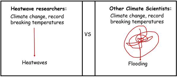
Talk about heatwaves and their impacts. This sounds really simple, but I’ve noticed a tendency of a proportion of climate scientists to talk about record breaking temperatures and never mention land heatwaves (For example the Royal Institute Christmas Lectures 2020). Some even make a wild leap from temperature straight to flooding, which is just painful for me as a heatwave researcher.
Figure 4: A schematic of heatwaves researchers and other climate scientists talking about climate change.
So let’s start by talking about heatwaves, heat stress and their impacts.
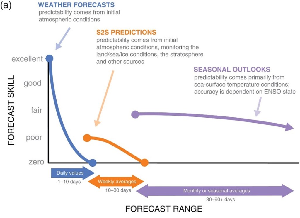
The February-March 2018 European cold-wave, known widely as “The Beast from the East” occurred around 2 weeks after a major sudden stratospheric warming (SSW) event on February 12th. Major SSWs typically occur once every other winter, involving significant disruption to the stratospheric polar vortex (a planetary-scale cyclone which resides over the pole in winter). SSWs are important because their occurrence can influence the type and predictability of surface weather on longer timescales of between 2 weeks to 2 months. This is known as subseasonal-to-seasonal (S2S) predictability, and “bridges the gap” between typical weather forecasts and seasonal forecasts (Figure 1).
Figure 1: Schematic of medium-range, S2S and seasonal forecasts and their relative skill. [Figure 1 in White et al. (2017)]
In general, S2S forecasts suffer from relatively low skill. While medium-range forecasts are an initial value problem (depending largely on the initial conditions of the forecast) and seasonal forecasts are a boundary value problem (depending on slowly-varying constraints to the predictions, such as the El Niño-Southern Oscillation), S2S forecasts lie somewhere between the two. However, certain “windows of opportunity” can occur that have the potential to increase S2S skill – and a major SSW is one of them. Skilful S2S forecasts can be of particular benefit to public health planners, the transport sector, and energy demand management, among many others.
Given that we know that following an SSW certain weather types are more likely for several weeks, and forecasts may be more skilful, it might seem advantageous to know an SSW was coming at a long lead-time in order to really push the boundaries of S2S prediction. So, what about in 2018?
In the first paper from my PhD, published in July 2019 in JGR-Atmospheres, we explored the onset of predictions of the February 2018 SSW. We found that, until about 12 days beforehand, extended-range forecasts that contribute to the S2S database (an international collaboration of extended-range forecast data) did not accurately predict the event; in fact, most predictions indicated the vortex would remain unusually strong!
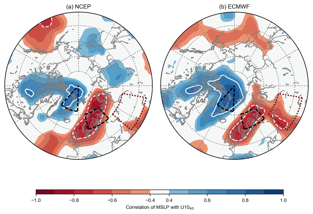
We diagnosed that anticyclonic wave breaking in the North Atlantic was a crucial synoptic-scale “trigger” event for perturbing the stratospheric vortex, by enhancing vertically propagating Rossby waves (which weaken the vortex when they break in the stratosphere). Forecasts struggled to predict this event far in advance, and thus struggled to predict the SSW. We called the pattern the “Scandinavia-Greenland (S-G) dipole” – characterised by an anticyclone over Scandinavia and a low over Greenland (Figure 2), and we found it was present before 35% of previous SSWs (1979-2018). The result agrees with several previous studies highlighting the role of blocking in the Scandinavia-Urals region, but was the first to suggest such a significant impact of a single tropospheric event.
Figure 2: Correlation between mean sea level pressure forecasts over 3-5 February 2018 and subsequent forecasts of 10 hPa 60°N zonal-mean zonal wind on 9-11 February, in (a) NCEP and (b) ECMWF ensembles launched between 29 January and 1 February 2018. White lines (dashednegative) indicate correlations exceeding +/- 0.7, while the black dashed lines indicate the nodes of the S-G dipole. [Figure 3 in Lee et al. (2019)]
So, we had established the S-G dipole was important in the predictability onset in 2018, and important in previous cases – but how well do S2S models generally capture the pattern?
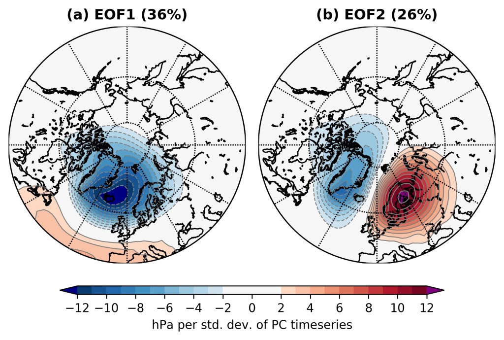
That was the subject of our recent (open-access) paper, published in August in QJRMS. We define a more generalised pattern by performing empirical orthogonal function (EOF) analysis on mean sea-level pressure anomalies in a region of the northeast Atlantic during November-March in ERA5 reanalysis (Figure 3). While the leading EOF (the “zonal pattern”) resembles the NAO, the 2nd EOF resembles the S-G dipole from our previous paper – so we call it the “S-G pattern”.
Figure 3:The first two leading EOFs of MSLP anomalies in the northeast Atlantic during November-March in ERA5, expressed as hPa per standard deviation of the principal component timeseries. The percentage of variance explained by the EOF is also shown. [Figure 1 in Lee et al. (2020)]
We then establish, through lagged linear regression analysis, that the S-G pattern is associated with enhanced vertically propagating wave activity (measured by zonal-mean eddy heat flux) into the stratosphere, and a subsequently weakened stratospheric vortex for the next 2 months. Thus, it supports our earlier work, and motivates considering how the pattern is represented in S2S models. To do this, we look at hindcasts – forecasts initialised for dates in the past – from 10 different prediction systems from around the world.
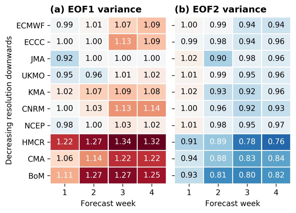
We find that while all the S2S models represent the spatial pattern of these two EOFs very well, some have biases in the variance explained by the EOFs, particularly at weeks 3 and 4 (Figure 4). Broadly, all the models have more variance explained by their first EOF compared with ERA5, and less by the second EOF – but this bias is particularly large for the three models with the lowest horizontal resolution (BoM, CMA, and HMCR).
Figure 4: Weekly-mean ratio between the variance explained by the EOFs in each model and the ERA5 EOF. [Figure 6 in Lee et al. (2020)]
Additionally, we find that the deterministic prediction skill in the S-G pattern (measured by the ensemble-mean correlation) can be as small as 5-6 days for the BoM model – and only as high as 11 days in the higher resolution models. Extending this to probabilistic skill in weeks 3 and 4, we find models have only limited (if any) skill above climatology in weeks 3 and 4 (and much less than the skill in the leading EOF, the NAO-like pattern).
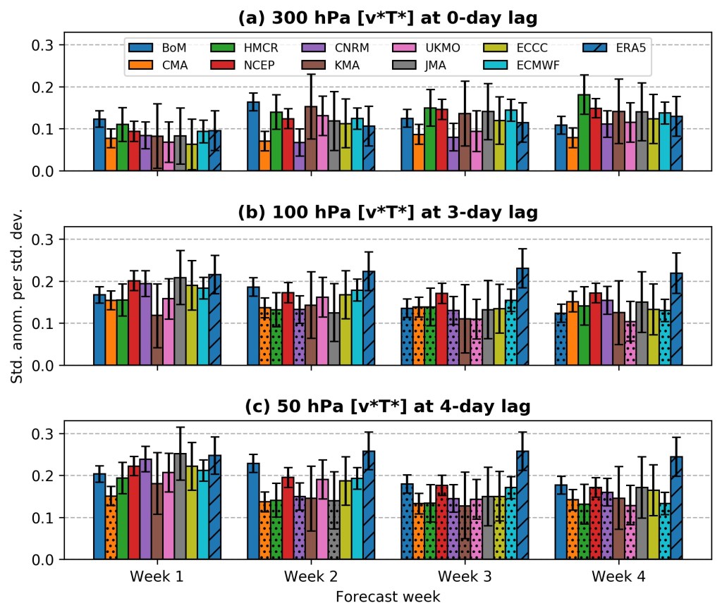
Furthermore, we find that the relationship between the S-G pattern and the enhanced heat flux in the stratosphere decays with lead-time in most S2S models, even in the higher-resolution models (Figure 5). Thus, this suggests that the dynamical link between the troposphere and stratosphere weakens with lead time in these models – so even a correct tropospheric prediction may not, in these cases, have a subsequently accurate extended-range stratospheric forecast.
Figure 5: Weekly meanregression coefficients between theS–G index and the correspondingeddy heat flux anomalies at (a) 300hPa on the same day, (b) 100 hPathree days later, and (c) 50 hPa fourdays later. The lags correspond todays with maximum correlation inERA5. Stippled bars indicate a significant difference from ERA5 at the 95% confidence level. [Figure 11 in Lee et al. (2020)]
So, when taking this all together, we have:
The S-G pattern is the second-leading mode of MSLP variability in the northeast Atlantic during winter.
It is associated with enhanced vertically propagating wave activity into the stratosphere and a weakened polar vortex in the following weeks to months.
S2S models represent the spatial patterns of the two leading EOFs well.
Most S2S models have a zonal variability bias, with relatively more variance explained by the leading EOF and correspondingly less in the second EOF.
This bias is largest in the lowest-resolution models in weeks 3 and 4.
Extended range skill in the S-G pattern is low, and lower than for the NAO-like zonal pattern.
The linear relationship between the S-G pattern and eddy heat flux in the stratosphere decays with lead-time in most S2S models.
The zonal variance bias is consistent with S2S model biases in Rossby wave breaking and blocking, while these biases have been widely found to be largest in the lowest resolution models. The results suggest that the poor prediction of the S-G event in February 2018 is not unique to that case, but a more generic issue. Overall, the combination of the variability biases, the poor extended-range predictability, and the poor representation of its impact on the stratospheric vortex at longer lead-times likely contributes to limiting skill at predicting major SSWs on S2S timescales – which remains low, despite the stratosphere’s much longer timescales. Correcting the biases outlined here will likely contribute to improving this skill, and subsequently increasing how far we are able to predict real-world weather.
To date, the 2020 North Atlantic hurricane season has been the most active on record, producing 20 named storms, 7 hurricanes, and a major hurricane which caused $9 billion in damages across the southern United States. With the potential for such destructive storms, it is understandable that a large amount of attention is paid to the North Atlantic basin at this time of year. Whilst hurricanes have been known to cause devastation in the tropics for centuries, until recently there was little appreciation for the destructive potential of these systems across Europe.
As tropical cyclones such as hurricanes move poleward – away from the tropics and into regions of lower sea surface temperatures and higher vertical wind shear, they undergo a process called extratropical transition (Klein et al., 2000): Over a period of time, the cyclones change from symmetric, warm cored systems into asymmetric cold core systems fuelled by horizontal temperature gradients, as opposed to latent heat fluxes (Evans et al., 2017). These systems, so-called post-tropical cyclones (PTCs), often reintensify in the mid-latitude Atlantic with consequences for land masses downstream – often Europe. This was highlighted in 2017, when ex-hurricane Ophelia impacted Ireland, bringing with it the strongest winds Ireland had seen in 50 years (Stewart, 2018). 3 people were killed, and 360,000 homes were without power.
In a recent paper, we quantify the risk associated with PTCs across Europe relative to mid-latitude cyclones (MLCs) for the first time – in terms of both the absolute risk (i.e. what fraction of high impact wind events across Europe are caused by PTCs?) and also the relative risk (for a given PTC, how likely is it to be associated with high-impact winds, and how does this compare to a given MLC?). By tracking all cyclones impacting a European domain (36-70N, 10W-30E) in the ERA5 reanalysis (1979-2017) using a feature tracking algorithm (Hodges, 1994, 1995, 1999), we identify the post-tropical cyclones using spatiotemporal matching (Hodges et al., 2017) with the observational record, IBTrACS (Knapp et al., 2010).
Figure 1: Distributions of the maximum intensity (maximum wind speed, minimum MSLP) attained by each PTC and MLC inside (a-c) the whole European domain (36-70N, 10W-30E), (d-f) the Northern Europe domain (48-70N, 10W-30E) and (g-i) the Southern Europe domain (36-48N, 10W-30E), using cyclones tracked through the ERA5 reanalysis all year round, 1979-2017. [Figure 2 in Sainsbury et al. 2020].
Figure 1 shows the distributions of maximum intensity for PTCs and MLCs across the entire European domain (top), Northern Europe (48-70°N, 10°W-30°E; middle) and Southern Europe (36-48°N, 10°W-30°E; bottom), using all cyclone tracks all year round. The distribution of PTC maximum intensities is higher (in terms of both wind speed and MSLP) than MLCs, particularly across Northern Europe. The difference between the maximum intensity distributions of PTCs and MLCs across Northern Europe is statistically significant (99%). PTCs are also present in the highest of intensity bins, indicating that the strongest PTCs have intensities comparable to strong wintertime MLCs.
Whilst Figure 1 shows that PTCs are stronger than MLCs even when considering MLCs forming all year round (including the often much stronger wintertime MLCs), it is also useful to compare the risks posed by PTCs relative to MLCs forming at the same time of the year – during the North Atlantic hurricane season (June 1st-November 30th).
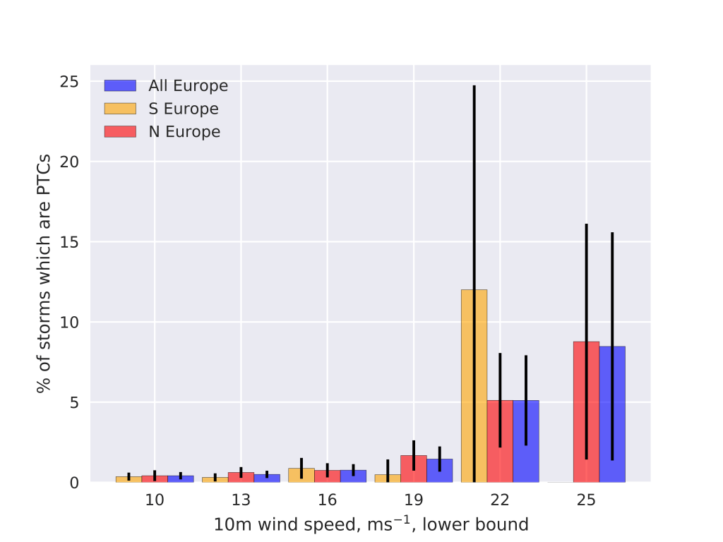
Figure 2 shows the fraction of all storms, binned by their maximum intensity in their respective domains, which are PTCs. For storms with weak-moderate maximum winds (first three bins in the figure), <1% of such events are caused by PTCs (with the remaining 99% caused by MLCs). For stronger storms, particularly those of storm force (>25 ms-1 on the Beaufort scale), this percentage is much higher. Despite less than 1% of all storms impacting Northern Europe during hurricane season being PTCs, almost 9% of all storms with storm-force winds which impact the region are PTCs, suggesting that a disproportionate fraction of high-impact windstorms are PTCs. 8.2% of all Northern Europe impacting PTCs which form during hurricane season impact the region with storm-force winds. This fraction is only 0.8% for MLCs, suggesting that the fraction of PTCs impacting Northern Europe with storm-force winds is approximately 10 times greater than MLCs.
Figure 2: The fraction of cyclones impacting Europe which are PTCs as a function of their maximum 10m wind speed in their respective domain. Lower bound of wind speed is shown on the x axis, bin width = 3. Error bars show the 95% confidence interval. All cyclone tracks forming during the North Atlantic hurricane season are used. [Figure 4 in Sainsbury et al. 2020].
Here we have shown that PTCs, at their maximum intensity over Northern Europe, are stronger than MLCs. However, the question still remains as to why this is the case. Warm-seclusion storms post-extratropical transition have been shown to have the fastest rates of reintensification (Kofron et al., 2010) and typically have the lowest pressures upon impacting Europe (Dekker et al., 2018). Given the climatological track that PTCs often take over the warm waters of the Gulf stream, along with the contribution of both baroclinic instability and latent heat release for warm-seclusion development (Baatsen et al., 2015), one hypothesis may be that PTCs are more likely to develop into warm seclusion storms than the broader class of mid-latitude cyclones, potentially explaining the disproportionate impacts they cause across Europe. This will be the topic of future work.
Despite PTCs disproportionately impacting Europe with high intensities, they are a relatively small component of the total cyclone risk in the current climate. However, only small changes are expected in MLC number and intensity under RCP 4.5 (Zappa et al., 2013). Conversely, the number of hurricane-force (>32.6 ms-1) storms impacting Norway, the North Sea and the Gulf of Biscay has been projected to increases by a factor of 6.5, virtually all of which originate in the tropics (Haarsma et al., 2013). Whilst the absolute contribution of PTCs to hurricane season windstorm risk is currently low, PTCs may make an increasingly significant contribution to European windstorm risk in a future climate.
Sainsbury, E. M., R. K. H. Schiemann, K. I. Hodges, L. C. Shaffrey, A. J. Baker, K. T. Bhatia, 2020: How Important Are Post‐Tropical Cyclones for European Windstorm Risk? Geophysical Research Letters, 47(18), e2020GL089853, https://doi.org/10.1029/2020GL089853
References
Baatsen, M., Haarsma, R. J., Van Delden, A. J., & de Vries, H. (2015). Severe Autumn storms in future Western Europe with a warmer Atlantic Ocean. Climate Dynamics, 45, 949–964. https://doi.org/10.1007/s00382-014-2329-8
Dekker, M. M., Haarsma, R. J., Vries, H. de, Baatsen, M., & Delden, A. J. va. (2018). Characteristics and development of European cyclones with tropical origin in reanalysis data. Climate Dynamics, 50(1), 445–455. https://doi.org/10.1007/s00382-017-3619-8
Evans, C., Wood, K. M., Aberson, S. D., Archambault, H. M., Milrad, S. M., Bosart, L. F., et al. (2017). The extratropical transition of tropical cyclones. Part I: Cyclone evolution and direct impacts. Monthly Weather Review, 145(11), 4317–4344. https://doi.org/10.1175/MWR-D-17-0027.1
Haarsma, R. J., Hazeleger, W., Severijns, C., De Vries, H., Sterl, A., Bintanja, R., et al. (2013). More hurricanes to hit western Europe due to global warming. Geophysical Research Letters, 40(9), 1783–1788. https://doi.org/10.1002/grl.50360
Hodges, K., Cobb, A., & Vidale, P. L. (2017). How well are tropical cyclones represented in reanalysis datasets? Journal of Climate, 30(14), 5243–5264. https://doi.org/10.1175/JCLI-D-16-0557.1
Klein, P. M., Harr, P. A., & Elsberry, R. L. (2000). Extratropical transition of western North Pacific tropical cyclones: An overview and conceptual model of the transformation stage. Weather and Forecasting, 15(4), 373–395. https://doi.org/10.1175/1520-0434(2000)015<0373:ETOWNP>2.0.CO;2
Knapp, K. R., Kruk, M. C., Levinson, D. H., Diamond, H. J., & Neumann, C. J. (2010). The international best track archive for climate stewardship (IBTrACS). Bulletin of the American Meteorological Society, 91(3), 363–376. https://doi.org/10.1175/2009BAMS2755.1
Kofron, D. E., Ritchie, E. A., & Tyo, J. S. (2010). Determination of a consistent time for the extratropical transition of tropical cyclones. Part I: Examination of existing methods for finding “ET Time.” Monthly Weather Review, 138(12), 4328–4343. https://doi.org/10.1175/2010MWR3180.1
Stewart, S. R. (2018). Tropical Cyclone Report: Hurricane Ophelia. National Hurricane Center, (February), 1–32. https://doi.org/AL142016
Zappa, G., Shaffrey, L. C., Hodges, K. I., Sansom, P. G., & Stephenson, D. B. (2013). A multimodel assessment of future projections of North Atlantic and European extratropical cyclones in the CMIP5 climate models. Journal of Climate, 26(16), 5846–5862. https://doi.org/10.1175/JCLI-D-12-00573.1
The Arctic sea ice cover is made up of discrete units of sea ice area called floes. The size of these floes has an impact on several sea ice processes including the volume of melt produced at floe edges, the momentum exchange between the sea ice, ocean, and atmosphere, and the mechanical response of the sea ice to stress. Models of the sea ice have traditionally assumed that floes adopt a uniform size, if floe size is explicitly represented at all in the model. Observations of floes show that floe size can span a huge range, from scales of metres to tens of kilometres. Generally, observations of the floe size distribution (FSD) are fitted to a power law or a combination of power laws (Stern et al., 2018a).
The Los Alamos sea ice model, hereafter referred to as CICE, usually assumes a fixed floe size of 300 m. We can impose a simple FSD model into CICE derived from a power law to explore the impact of variable floe size on the sea ice cover. Figure 1 is a diagram of the WIPoFSD model (Waves-in-Ice module and Power law Floe Size Distribution model), which assumes a power law with a fixed exponent, , between a lower floe size cut-off, , and an upper floe size cut-off, . The model also incorporates a floe size variable, , to capture the effects of processes that can influence floe size. The processes represented are wave break-up of floes, melting at the floe edge, winter floe growth, and advection. The model includes a wave advection and attenuation scheme so that wave properties can be determined within the sea ice field to enable the identification of wave break-up events. Full details of the WIPoFSD model and its implementation into CICE are available in Bateson et al. (2020). For the WIPoFSD model setup considered here, we explore the impact of the FSD on the lateral melt rate, which is the melt rate at the edge surfaces of floes. It is useful to define a new FSD metric that can be used to characterise the impact of the FSD on lateral melt. To do this we note that the lateral melt volume produced by a floe is proportional to the perimeter of the floe. The effective floe size, , is defined as a fixed floe size that would produce the same lateral melt rate as a given FSD, for a fixed total sea ice area.
Figure 1: A schematic of the imposed FSD model. This model is initiated by prescribing a power law with an exponent, , and between the limits and . Within individual grid cells the variable FSD tracer, , varies between these two limits. evolves through lateral melting, wave break-up events, freezing, and advection.
Here we will compare a CICE simulation incorporating the WIPoFSD model, hereafter referred to as stan-fsd, to a reference case, ref, using the CICE standard fixed floe size of 300 m. For the WIPoFSD model, = 10 m, = 30 km, and = -2.5. These values have been selected as representative values from observations. The reference setup is initiated in 1990 and spun-up until 2005, when either continued as ref or the WIPoFSD model imposed for stan-fsd before being evaluated from 2006 – 2016. All figures in this post are given as a mean over 2007 – 2016, such that 2005 – 2006 is a period of spin-up for the incorporated WIPoFSD model.
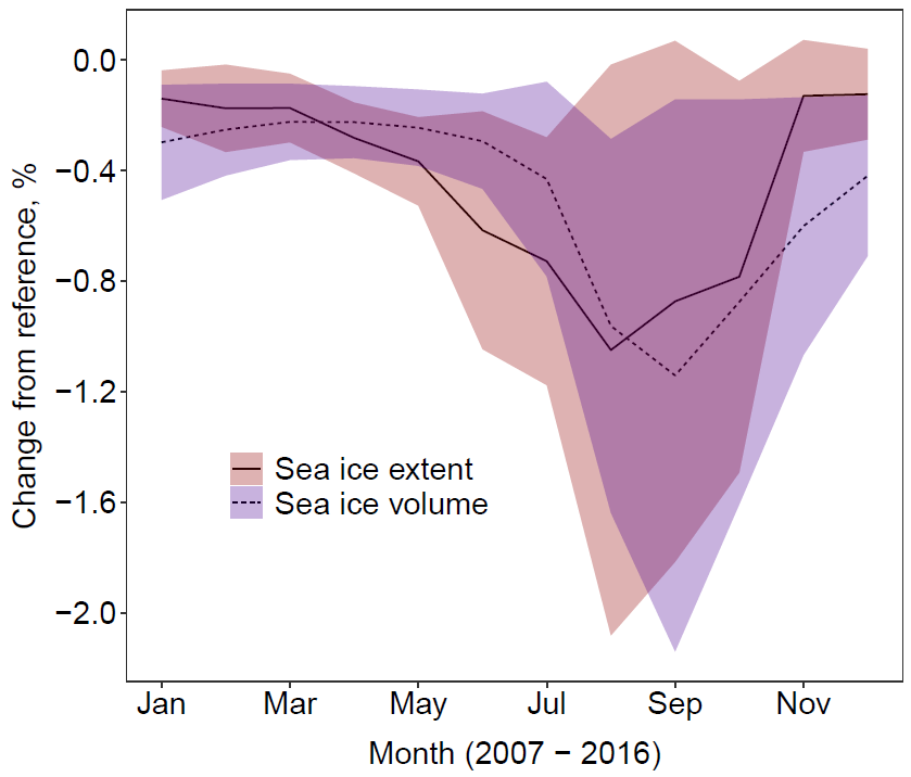
In Figure 2, we show the percentage reduction in the Arctic sea ice extent and volume of stan-fsd relative to ref. The differences in both extent and volume over the pan-Arctic scale evolve over an annual cycle, with maximum differences of -1.0 % in August and -1.1 % in September respectively. The annual cycle corresponds to periods of melting and freeze-up and is a product of the nature of the imposed FSD. Lateral melt rates are a function of floe size, but freeze-up rates are not, hence model differences only increase during periods of melting and not during periods of freeze-up. The difference in sea ice extent reduces rapidly during freeze-up because this freeze-up is predominantly driven by ocean surface properties, which are strongly coupled to atmospheric conditions in areas of low sea ice extent. In comparison, whilst atmospheric conditions initiate the vertical sea ice growth, this atmosphere-ocean coupling is rapidly lost due to insulation of the warmer ocean from the cooler atmosphere once sea ice extends across the horizontal plane. Hence a residual difference in sea ice thickness and therefore volume propagates throughout the winter season. The interannual variability shows that the impact of the WIPoFSD model with standard parameters varies significantly depending on the year.
Figure 2: Difference in sea ice extent (solid, red ribbon) and volume (dashed, blue ribbon) between stan-fsd relative to ref averaged over 2007–2016. The ribbon shows the region spanned by the mean value plus or minus 2 times the standard deviation for each simulation. This gives a measure of the interannual variability over the 10-year period.
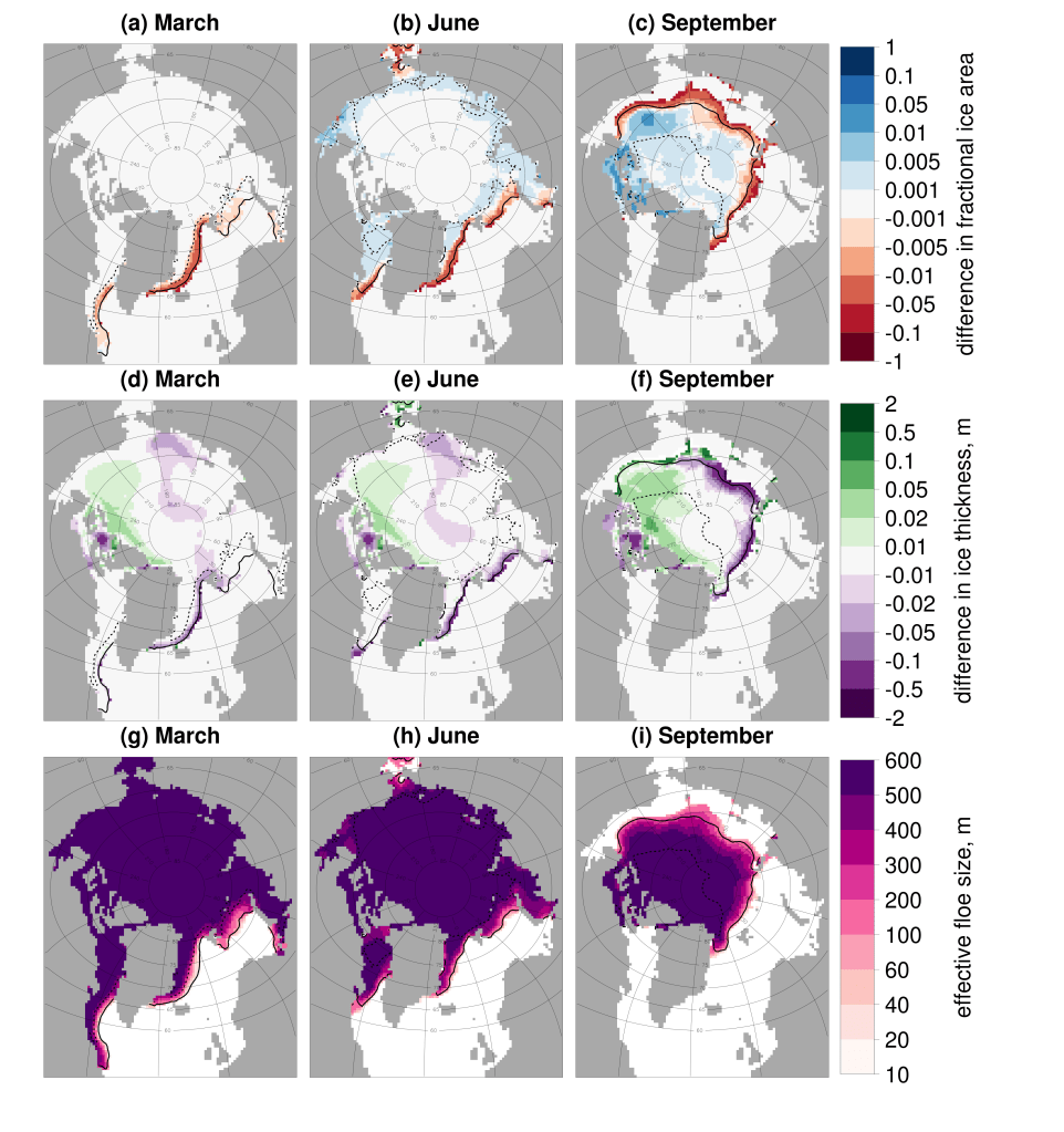
Although the pan-Arctic differences in extent and volume shown in Figure 2 are marginal, differences are larger when considering smaller spatial scales. Figure 3 shows the spatial distribution in the changes in sea ice concentration and thickness in March, June, and September for stan-fsd relative to ref in addition to the spatial distribution in for stan-fsd for the same months. Reductions in the sea ice concentration and thickness of up to 0.1 and 50 cm observed respectively in the September marginal ice zone (MIZ). Within the pack ice, increases in the sea ice concentration of up to 0.05 and ice thickness of up to 10 cm can be seen. To understand the non-uniform spatial impacts of the FSD, it is useful to look at the behaviour of . Regions with an greater than 300 m will experience less lateral melt than the equivalent location in ref (all other things being equal) whereas locations with an below 300 m will experience more lateral melt. In Figure 3 we see the transition to values of smaller than 300 m in the MIZ, hence most of the sea ice cover experiences less lateral melting for stan-fsd compared to ref.
Figure 3: Difference in the sea ice concentration (top row, a-c) and thickness (middle row, d-f) between stan-fsd and ref and (bottom row, g-i) for stan-fsd averaged over 2007 – 2016. Results are presented for March (left column, a, d, g), June (middle column, b, e, h) and September (right column, c, f, i). Values are shown only in locations where the sea ice concentration exceeds 5 %.
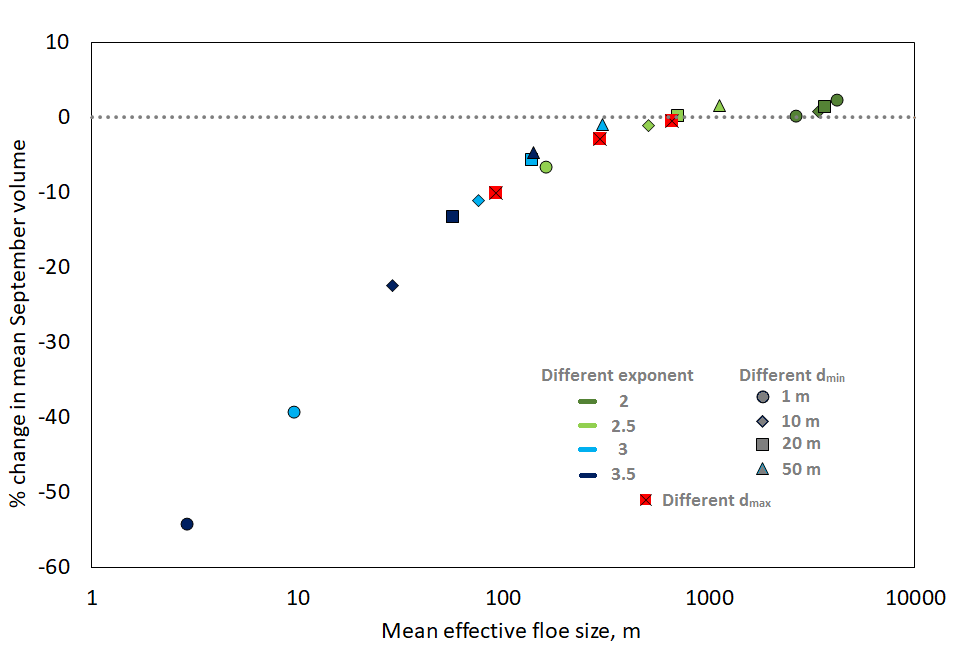
For Figures 2-3, the parameters used to define the FSD have been set to fixed, standard values. However, these parameters vary significantly between different observed FSDs. It is therefore useful to explore the model sensitivity to these parameters. For α values of -2, -2.5, -3 and -3.5 have been selected to span the general range of values reported in observations (Stern et al., 2018a). For values of 1 m, 20 m and 50 m are selected to reflect the different behaviours reported in studies, with some showing power law behaviour extending to 1 m (Toyota et al., 2006) and others showing a tailing off at an order of 10 s of metres (Stern et al., 2018b). For the upper cut-off, , values of 1000 m, 10,000 m, 30,000 m and 50,000 m are selected, again to represent the distributions reported in different studies. 50 km is taken as the largest value for as this serves as an upper limit to what can be resolved within an individual grid cell on a CICE 1 grid. A total of 19 sensitivity studies have been completed used different permutations of the stated values for the FSD model parameters. Figure 4 shows the change in mean September sea ice extent and volume relative to ref plotted against mean annual , averaged over the sea ice extent, for each of these sensitivity studies. The impacts range from a small increase in extent and volume to large reductions of -22 % and -55 % respectively, even within the parameter space defined by observations. Furthermore, there is almost a one-to-one mapping between mean and extent and volume reduction. This suggests is a useful diagnostic tool to predict the impact of a given set of floe size parameters. The system varies most in response to the changes in the α, but it is also particularly sensitive to .
Figure 4: Relative change (%) in mean September sea ice volume from 2007 – 2016 respectively, plotted against mean for simulations with different selections of parameters relative to ref. The mean is taken as the equally weighted average across all grid cells where the sea ice concentration exceeds 15%. The colour of the marker indicates the value of the , the shape indicates the value of , and the three experiments using standard parameters but different (1000 m, 10000 m and 50000 m) are indicated by a crossed red square. The parameters are selected to be representative of a parameter space for the WIPoFSD model that has been constrained by observations.
There are several advantages to the assumption of a fixed power law in modelling the sea ice floe size distribution. It provides a simple framework to explore the potential impact of an observed FSD on the sea ice mass balance, given observations of the FSD are generally fitted to a power law. In addition, the use of a simple model makes it easier to constrain the mechanism of how the model changes the sea ice cover. However, there are also significant disadvantages including the high model sensitivity to poorly constrained parameters, as shown in Figure 4. In addition, there is evidence both that the exponent evolves over an annual cycle and is not a fixed value (Stern et al., 2018b) and that the power law is not a statistically valid description of the FSD over all floe sizes (Horvat et al., 2019). An alternative approach to modelling the FSD is the prognostic model of Roach et al. (2018, 2019). The prognostic model avoids any assumptions about the shape of the distribution and instead assigns sea ice area to a set of adjacent floe size categories, with individual processes parameterised at floe scale. This approach carries its own set of challenges. If important physical processes are missing from the model it will not be possible to simulate a physically realistic distribution. In addition, the prognostic model has a significant computational cost. In practice, the choice of FSD modelling approach will depend on the application.
Further reading Bateson, A. W., Feltham, D. L., Schröder, D., Hosekova, L., Ridley, J. K. and Aksenov, Y.: Impact of sea ice floe size distribution on seasonal fragmentation and melt of Arctic sea ice, Cryosphere, 14, 403–428, https://doi.org/10.5194/tc-14-403-2020, 2020.
Horvat, C., Roach, L. A., Tilling, R., Bitz, C. M., Fox-Kemper, B., Guider, C., Hill, K., Ridout, A., and Shepherd, A.: Estimating the sea ice floe size distribution using satellite altimetry: theory, climatology, and model comparison, The Cryosphere, 13, 2869–2885, https://doi.org/10.5194/tc-13-2869-2019, 2019.
Stern, H. L., Schweiger, A. J., Zhang, J., and Steele, M.: On reconciling disparate studies of the sea-ice floe size distribution, Elem. Sci. Anth., 6, p. 49, https://doi.org/10.1525/elementa.304, 2018a.
Stern, H. L., Schweiger, A. J., Stark, M., Zhang, J., Steele, M., and Hwang, B.: Seasonal evolution of the sea-ice floe size distribution in the Beaufort and Chukchi seas, Elem. Sci. Anth., 6, p. 48, https://doi.org/10.1525/elementa.305, 2018b.
Roach, L. A., Horvat, C., Dean, S. M., and Bitz, C. M.: An Emergent Sea Ice Floe Size Distribution in a Global Coupled Ocean-Sea Ice Model, J. Geophys. Res.-Oceans, 123, 4322–4337, https://doi.org/10.1029/2017JC013692, 2018.
Roach, L. A., Bitz, C. M., Horvat, C. and Dean, S. M.: Advances in Modeling Interactions Between Sea Ice and Ocean Surface Waves, J. Adv. Model. Earth Syst., 11, 4167–4181, https://doi.org/10.1029/2019MS001836, 2019.
Toyota, T., Takatsuji, S., and Nakayama, M.: Characteristics of sea ice floe size distribution in the seasonal ice zone, Geophys. Res. Lett., 33, 2–5, https://doi.org/10.1029/2005GL024556, 2006.
Downward trends in Arctic sea-ice extent in recent decades are a striking signal of our warming planet. Loss of sea ice has major implications for future climate because it strongly influences the Earth’s energy budget and plays a dynamic role in the atmosphere and ocean circulation.
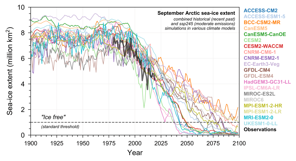
Comprehensive numerical models are used to make long-term projections of the future climate state under different greenhouse gas emission scenarios. They estimate that the Arctic ocean will become seasonally ice free by the end of the 21st century, but there is a large uncertainty on the timing due to the spread of estimates across models (Fig. 1).
What causes this spread, and how might it be reduced to better constrain future projections? There are various factors (Notz et al. 2016), but of interest to our work is the large-scale forcing of the atmosphere and ocean. The mean atmospheric circulation transports about 3 PW of heat from lower latitudes into the Arctic, and the oceans transport about a tenth of that (e.g. Trenberth and Fasullo, 2017; 1 PW = 1015 W). Our goal is to understand the relative roles of Ocean and Atmospheric Heat Transports (OHT, AHT) on long timescales. Specifically, how sensitive is the sea-ice cover to deviations in OHT and AHT, and what underlying mechanisms determine the sensitivities?
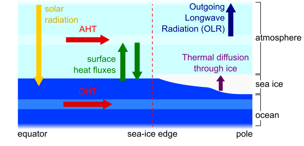
We developed a highly simplified Energy-Balance Model (EBM) of the climate system (Fig. 2)—it has only latitudinal variations and is described by a few simple equations relating energy transfer between the atmosphere, ocean, and sea ice (Aylmer et al. 2020). The latitude of the sea-ice edge is an analogue for ice extent in the real world. The simplicity of the EBM allows us to isolate the basic physics of the problem, which would not be possible going directly with the complex output of a full climate model.
Figure 2: Simplified schematic of our Energy-Balance Model (EBM; see Aylmer et al. 2020 for technical details). Arrows represent energy fluxes, each varying with latitude, between the atmosphere, ocean, and sea ice.
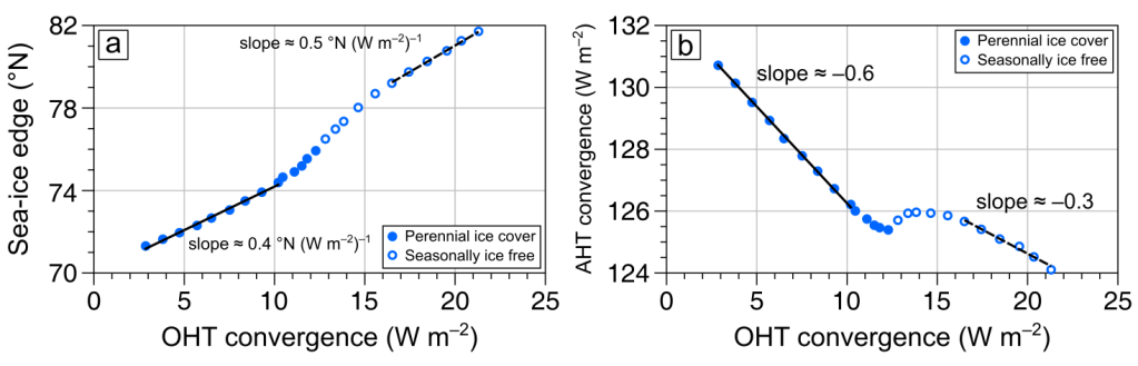
We generated a set of simulations in which OHT varies and checked the response of the ice edge. This is a measure of the effective sensitivity of the ice cover to OHT (Fig. 3a)—it is not the actual sensitivity because AHT decreases (Fig. 3b), and we are really seeing in Fig. 3a the net response of the ice edge to changes in both OHT and AHT.
Figure 3: (a) Effective sensitivity of the (annual-mean) sea-ice edge to varying OHT (expressed as the mean convergence over the ice pack). (b) AHT convergence reduces at the same time, which partially cancels the true impact of increasing OHT on sea ice.
This reduction in AHT with increasing OHT is called Bjerknes compensation, and it occurs in full climate models too (Outten et al. 2018). Here, it has a moderating effect on the true impact of increasing OHT. With further analysis, we determined the actual sensitivity to be about 1.5 times the effective sensitivity. The actual sensitivity of the ice edge to AHT turns out to be about half that to the OHT.
What sets the difference in OHT and AHT sensitivities? This is easily answered within the EBM framework. We derived a general expression for the ratio of (actual) ice-edge sensitivities to OHT (so) and AHT (sa):
A higher-order term has been neglected for simplicity here, but the basic point remains: the ratio of sensitivities mainly depends on the parameters BOLR and Bdown. These are bulk representations of atmospheric feedbacks and determine the efficiency of outgoing and downwelling longwave radiation, respectively. They are always positive, so the ice edge is always more sensitive to OHT than AHT.
The interpretation of this equation is simple. AHT converging over the ice pack can either be transferred to the underlying sea ice, or radiated to space, having no impact on the ice, and the partitioning is controlled by Bdown and BOLR. The same amount of OHT converging under the ice pack can only go through the ice and is thus the more efficient driver.
Climate models with larger OHTs tend to have less sea ice (Mahlstein and Knutti, 2011). We have also found strong correlations between OHT and the sea-ice edge in several of the models listed in Fig. 1 individually. Ice-edge sensitivities and B values can be determined per model, and our equation predicts how these should be related. Our work thus provides a way to investigate how much physical biases in OHT and AHT contribute to sea-ice-projection uncertainties.
 is vertically-integrated FMSE,
  and
and  are the net atmospheric column longwave and shortwave heating rates,
  is the surface enthalpy flux, made up of the surface latent and sensible heat fluxes, and
  is the horizontal divergence of the
  ) indicate local anomalies from the instantaneous domain mean. The subscript (
 ) denotes a normalised variable which is the original variable divided by the difference between the hypothetical upper and lower limits of
  variance (left hand side term) is driven by interactions between
  anomalies and anomalies in normalised net longwave heating, shortwave heating, surface fluxes and advection.


 and
and  . We can see
  are closely correlated since
 and
and  and the Mature phase has
  and
and  . The contribution of longwave interactions with each cloud type to aggregation during these two phases is shown in Figure 5a, with their mean
  covariance and fraction shown in Figures 5b & c.


 , between a lower floe size cut-off,
  , and an upper floe size cut-off,
  . The model also incorporates a floe size variable,
  , to capture the effects of processes that can influence floe size. The processes represented are wave break-up of floes, melting at the floe edge, winter floe growth, and advection. The model includes a wave advection and attenuation scheme so that wave properties can be determined within the sea ice field to enable the identification of wave break-up events. Full details of the WIPoFSD model and its implementation into CICE are available in Bateson et al. (2020). For the WIPoFSD model setup considered here, we explore the impact of the FSD on the lateral melt rate, which is the melt rate at the edge surfaces of floes. It is useful to define a new FSD metric that can be used to characterise the impact of the FSD on lateral melt. To do this we note that the lateral melt volume produced by a floe is proportional to the perimeter of the floe. The effective floe size,
  , is defined as a fixed floe size that would produce the same lateral melt rate as a given FSD, for a fixed total sea ice area.
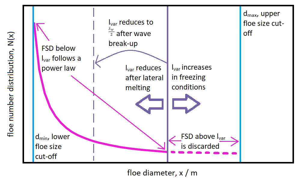
 grid. A total of 19 sensitivity studies have been completed used different permutations of the stated values for the FSD model parameters. Figure 4 shows the change in mean September sea ice extent and volume relative to ref plotted against mean annual