The Social Metwork

James Fallon – j.fallon@pgr.reading.ac.uk

As researchers, we familiarise ourselves with many different datasets. Depending on who put together the dataset, the variable names and definitions that we are already familiar from one dataset may be different in another. These differences can range from subtle annoyances to large structural differences, and it’s not always immediately obvious how best to handle them.

One dataset might be on an hourly time-index, and the other daily. The grid points which tell us the geographic location of data points may be spaced at different intervals, or use entirely different co-ordinate systems!

However most modern datasets come with hidden help in the form of metadata – this information should tell us how the data is to be used, and with the right choice of python modules we can use the metadata to automatically work with different datasets whilst avoiding conversion headaches.

First attempt…

Starting my PhD, my favourite (naïve, inefficient, bug prone,… ) method of reading data with python was with use of the built-in function open() or numpy functions like genfromtxt(). These are quick to set up, and can be good enough. But as soon as we are using data with more than one field, complex coordinates and calendar indexes, or more than one dataset, this line of programming becomes unwieldy and disorderly!

>>> header = np.genfromtxt(fname, delimiter=',', dtype='str', max_rows=1)
>>> print(header)
['Year' 'Month' 'Day' 'Electricity_Demand']
>>> data = np.genfromtxt(fnam, delimiter=',', skip_header=1)
>>> print(data)
array([[2.010e+03, 1.000e+00, 1.000e+00, 0.000e+00],
       [2.010e+03, 1.000e+00, 2.000e+00, 0.000e+00],
       [2.010e+03, 1.000e+00, 3.000e+00, 0.000e+00],
       ...,
       [2.015e+03, 1.200e+01, 2.900e+01, 5.850e+00],
       [2.015e+03, 1.200e+01, 3.000e+01, 6.090e+00],
       [2.015e+03, 1.200e+01, 3.100e+01, 6.040e+00]])

The above code reads in year, month, day data in the first 3 columns, and Electricity_Demand in the last column.

You might be familiar with such a workflow – perhaps you have refined it down to a fine art!

In many cases this is sufficient for what we need, but making use of already available metadata can make the data more readable, and easier to operate on when it comes to complicated collocation and statistics.

Enter pandas!

Pandas

In the previous example, we read in our data to numpy arrays. Numpy arrays are very useful, because they store data more efficiently than a regular python list, they are easier to index, and have many built in operations from simple addition to niche linear algebra techniques.

We stored column labels in an array called header, but this means our metadata has to be handled separately from our data. The dates are stored in three different columns alongside the data – but what if we want to perform an operation on just the data (for example add 5 to every value). It is technically possible but awkward and dangerous – if the column index changes in future our code might break! We are probably better splitting the dates into another separate array, but that means more work to record the column headers, and an increasing number of python variables to keep track of.

Using pandas, we can store all of this information in a single object, and using relevant datatypes:

>>> data = pd.read_csv(fname, parse_dates=[['Year', 'Month', 'Day']], index_col=0)
>>> data
Electricity_Demand
Year_Month_Day      
2010-01-01      0.00
2010-01-02      0.00
2010-01-03      0.00
2010-01-04      0.00
2010-01-05      0.00
...              ...
2015-12-27      5.70
2015-12-28      5.65
2015-12-29      5.85
2015-12-30      6.09
2015-12-31      6.04

[2191 rows x 1 columns]

This may not immediately appear a whole lot different to what we had earlier, but notice the dates are now saved in datetime format, whilst being tied to the data Electricity_Demand. If we want to index the data, we can simultaneously index the time-index without any further code (and possible mistakes leading to errors).

Pandas also makes it really simple to perform some complicated operations. In this example, I am only dealing with one field (Electricity_Demand), but this works with 10, 100, 1000 or more columns!

• Flip columns with data.T
• Calculate quantiles with data.quantile
• Cut to between dates, eg. data.loc['2010-02-03':'2011-01-05']
• Calculate 7-day rolling mean: data.rolling(7).mean()

We can insert new columns, remove old ones, change the index, perform complex slices, and all the metadata stays stuck to our data!

Whilst pandas does have many maths functions built in, if need-be we can also export directly to numpy using numpy.array(data['Electricity_Demand']) or data.to_numpy().

Pandas can also simplify plotting – particularly convenient when you just want to quickly visualise data without writing import matplotlib.pyplot as plt and other boilerplate code. In this example, I plot my data alongside its 7-day rolling mean:

ax = data.loc['2010'].plot(label='Demand', ylabel='Demand (GW)')
data.loc['2010'].rolling(7).mean().plot(ax=ax, label='Demand rolling mean')
ax.legend()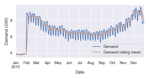

Now I can visualise the anomalous values at the start of the dataset, a consistent annual trend, a diurnal cycle, and fairly consistent behaviour week to week.

Big datasets

Pandas can read from and write to many different data formats – CSV, HTML, EXCEL, … but some filetypes like netCDF4 that meteorologists like working with aren’t built in.

xarray is an extremely versatile tool that can read in many formats including netCDF, GRIB. As well as having built in functions to export to pandas, xarray is completely capable of handling metadata on its own, and many researchers work directly with objects such as xarray DataArray objects.

There are more xarray features than stars in the universe^{[citation needed]}, but some that I find invaluable include:

open_mfdataset – automatically merge multiple files (eg. for different dates or locations)
assign_coords – replace one co-ordinate system with another
where – replace xarray values depending on a condition

Yes you can do all of this with pandas or numpy. But you can pass metadata attributes as arguments, for example we can get the latitude average with my_data.mean('latitude'). No need to work in indexes and hardcoded values – xarray can do all the heavy lifting for you!

Have more useful tips for working effectively with meteorological data? Leave a comment here or send me an email j.fallon@pgr.reading.ac.uk 🙂