Piyali Goswami: p.goswami@pgr.reading.ac.uk
Mehzooz Nizar: m.nizar@pgr.reading.ac.uk
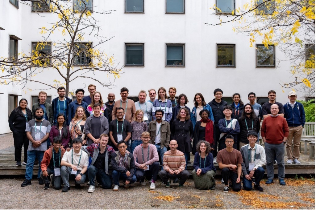
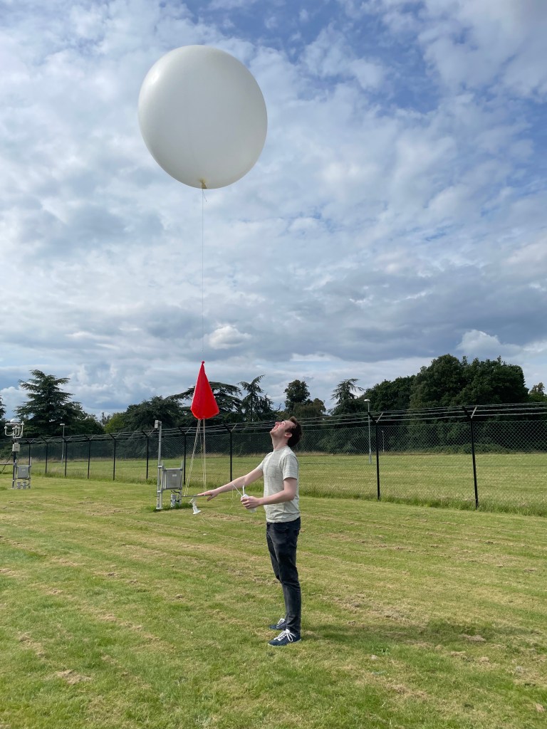
This September, we attended the NCAS Climate Modelling Summer School (CMSS), held at the University of Cambridge from 8th to 19th September. Five of us from the University of Reading joined this two-week residential programme. It was an intense and inspiring experience, full of lectures, coding sessions, discussions, and social events. In this blog, we would like to share our experiences.
About NCAS CMSS
The NCAS Climate Modelling Summer School (CMSS) is a visionary program, launched in 2007 with funding originating from grant proposals led by Prof. Pier Luigi Vidale. Run by leading researchers from the National Centre for Atmospheric Science and the University of Reading, it’s an immersive, practice-driven program that equips early-career researchers and PhD students with deeper expertise in climate modelling, Earth system science, and state-of-the-art computing. Held biennially in Cambridge, CMSS has trained 350 students from roughly 40 countries worldwide.
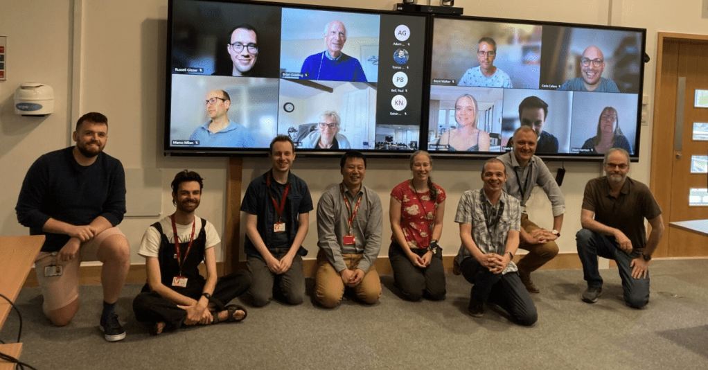
The CMSS 2025 brought together around 30 participants, including PhD students and professionals interested in the field of Climate Modelling.
Long Days, Big Ideas: Inside Our Schedule
The school was full of activity from morning to evening. We started around 9:00 AM and usually wrapped up by 8:30 PM, with a good mix of lectures, practical sessions, and discussions that made the long days fly by.
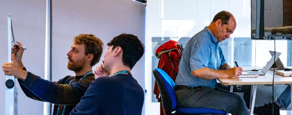
Week 1 was led by Dr Hilary Weller, who ran an excellent series on Numerical Methods for Atmospheric Models. Mornings were devoted to lectures covering core schemes; afternoons shifted to hands-on Python sessions to implement and test the methods. Between blocks, invited talks from leading researchers across universities highlighted key themes in weather and climate modelling. After dinner, each day closed with a thought-provoking discussion on climate modelling, chaired by Prof. Pier Luigi Vidale, where participants shared ideas on improving models and their societal impact.
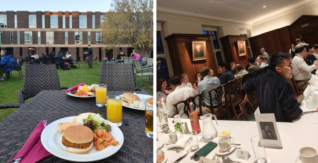
The week concluded with group presentations summarising the key takeaways from Hilary’s sessions and our first collaborative activity that set the tone for the rest of the school. It was followed by a relaxed barbecue evening, where everyone finally had a chance to unwind, chat freely, and celebrate surviving our first week together.
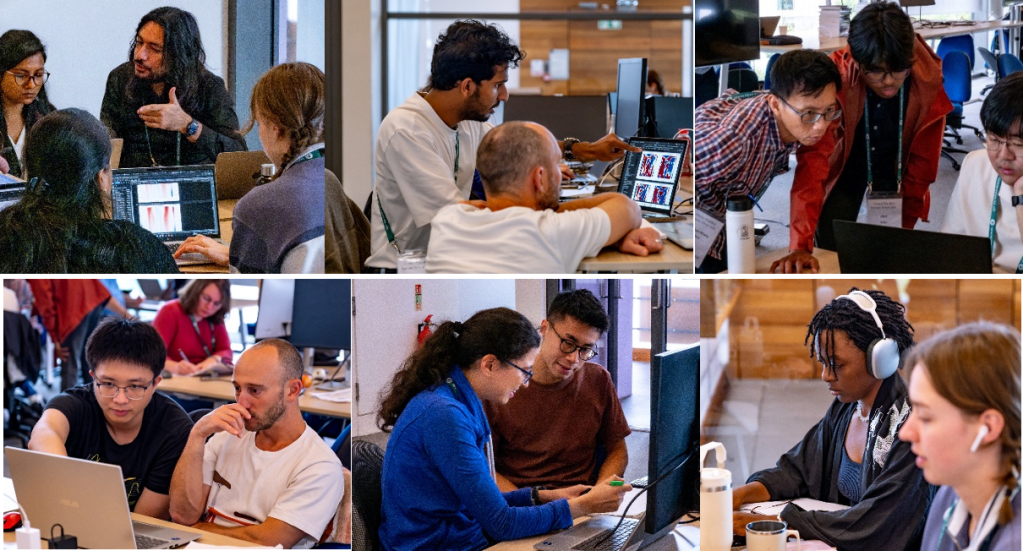
Week 2 was all about getting hands-on with a climate model and learning how to analyse its output. We moved into group projects using SpeedyWeather.jl to design and run climate model experiments. It is a global atmospheric model with simplified physics, designed as a research playground. One of the developers of SpeedyWeather.jl, Milan Klöwer, was with us throughout the week to guide and support our work. Each team explored a different question, from sensitivity testing to analysing the model outputs, and spent the afternoons debugging, plotting, and comparing results. Evenings featured talks from leading scientists on topics such as the hydrological cycle, land and atmosphere interactions, and the carbon cycle.
The week also included a formal dinner at Sidney Sussex, a welcomed pause before our final presentations. On Friday 19th of September, every group presented its findings before we all headed home. Some slides were finished only seconds before presenting, but the atmosphere was upbeat and supportive. It was a satisfying end to two weeks of hard work, shared learning, and plenty of laughter. A huge thank you to the teaching team for being there, from the “silly” questions to the stubborn bugs. Your patience, clarity, and genuine care made all the difference.
Coffee, Culture, and Climate Chat
The best part of the summer school was the people. The group was diverse: PhD students, and professionals from different countries and research areas. We spent nearly every moment together, from breakfast to evening socials, often ending the day with random games of “Would You Rather” or talking about pets. The summer school’s packed schedule brought us closer and sparked rich chats about science and life, everything from AI’s role in climate modelling to the policy levers behind climate action. We left with a lot to think about. Meeting people from around the world exposed us to rich cultural diversity and new perspectives on how science is practiced in different countries, insights that were both fresh and valuable. It went beyond training: we left with skills, new friends, and the seeds of future collaborations, arguably the most important part of research.
Reflections and takeaways
We didn’t become expert modellers in two weeks, but we did get a glimpse of how complex and creative climate modelling can be. The group presentations were chaotic but fun. Different projects, different approaches, and a few slides that weren’t quite finished in time. Some of us improvised more than we planned, but the atmosphere was supportive and full of laughter. More than anything, we learned by doing and by doing it together. The long days, the discussions, and the teamwork made it all worthwhile.
If you ever get the chance to go, take it. You’ll come back with new ideas, good memories, and friends who make science feel a little more human.
For the future participants
The NCAS CMSS usually opens in early spring, with applications closing around June. With limited spots, selection is competitive and merit-based, evaluating both fit for the course and the expected benefit to the student.
Bring curiosity, enthusiasm, and a healthy dose of patience, you’ll need all three. But honestly, that’s what makes it fun. You learn quickly, laugh a lot, and somehow find time to celebrate when a script finally runs without error. By the end, you’ll be tired, happy, and probably a little proud of how much you managed to do (and probably a few new friends who helped you debug along the way).


 (100 m) horizontal grid length, interesting dynamics emerge that have significant implications for urban air quality.
 is the flux of pollution,
  is the pollution concentration,
  is a turbulent diffusion coefficient and
  is the height from the ground.
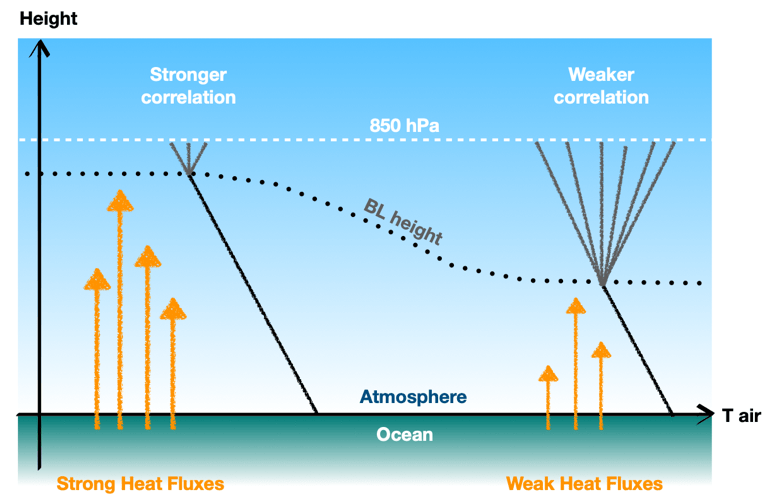
  is the non-local term which represents vertical turbulent mixing under convective conditions due to buoyant thermals (Lock et al., 2000; Siebesma et al., 2007).
  ) parametrisation of turbulent dispersion is consistent mathematically with Fickian diffusion of particles in a fluid. If
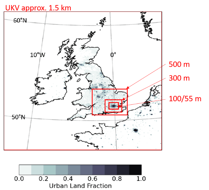
 7 ms-1) and the time at which there was most scalar in the upper BL compared to the lower BL in the puff release simulations (