The Social Metwork

Lily Greig – l.greig@pgr.reading.ac.uk

A week-long summer school on forecast verification was held jointly at the end of June by the MPECDT (Mathematics of Planet Earth Centre for Doctoral Training) and JWGFVR (Joint Working Group on Forecast Verification Research). The school featured lectures from scientists and academics from many different countries around the world including Brazil, USA and Canada. They each specialised in different topics within forecast verification. Participants gained a large overview of the field and how the fields within it interact.

Structure of school

The virtual school consisted of lectures from individual members of the JWGFVR on their own subjects, along with drop-in sessions for asking questions and dedicated time to work on group projects. Four groups of 4-5 students were given an individual forecast verification challenge. The themes of the projects were precipitation forecasts, comparing high resolution global model and local area model wind speed forecasts, and ensemble seasonal forecasts. The latter was the topic of our project.

Content

The first lecture was given by Barbara Brown, who provided a broad summary of verification and gave examples of questions that verifiers may ask themselves as they attempt to assess the “goodness” of a forecast. The next day, a lecture by Barbara Casati covered continuous scores (verification of continuous variables e.g., temperature), such as linear bias, mean-squared error (MSE) and Pearson coefficient. She also outlined the deficits of different scores and how it is best to use a variety of them when assessing the quality of a forecast. Marion Mittermaier then spoke about categorical scores (yes/no events or multi category events such as precipitation type). She gave examples such as contingency tables which portray how well a model is able to predict a given event, based on hit rates (how often the model predicted an event when the event happened), and false alarm rates (how often the model predicted the event when it didn’t happen). Further lectures were given by Ian Joliffe on methods of determining the significance of your forecast scores, Nachiketa Acharya on probabilistic scores and ensembles, Caio Coelho on sub-seasonal to seasonal timescales, and then Raghavendra Ashrit, Eric Gilleland and Caren Marzban on severe weather, spatial verification and experimental design. The lectures have been made available online and you can find them here.

Forecast Verification

So, forecast verification is as it sounds: a part of assessing the ‘goodness’ of a forecast as opposed to its value. Verification is helpful for economic purposes (e.g. decision making), as well as administrative and scientific ones (e.g. identifying model flaws). The other aspect of measuring how well a forecast is performing is knowing the user’s needs, and therefore how to apply the forecast. It is important to consider the goal of your verification process beforehand, as it will outline your choice of metrics and your assessment of them. An example of how forecast goodness hinges on the user was given by Barbara in her talk: a precipitation forecast may have a spatial offset of where a rain patch falls, but if both observation and forecast fall along the flight path, this may be all the aviation traffic strategic planner needs to know. For a watershed manager on the ground, however, this would not be a helpful forecast. The lecturers also emphasised the importance of performing many different measures on a forecast and then understanding the significance of your measures in order to help you understand its overall goodness. Identifying standards of comparison for your forecast is also important, such as persistence or climatology. Then there are further challenges such as spatial verification, which requires methods of ‘matching’ the location of your observations with the model predictions on the model grid.

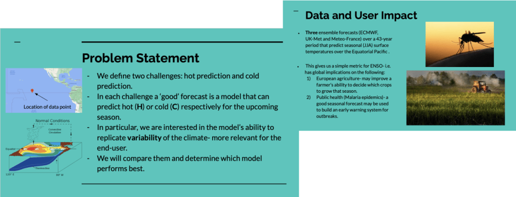
Figure 1: Problem statement for group presentation on 2m temperature ensemble seasonal forecasts, presented by Ryo Kurashina

Group Project

Our project was on verification of 2 metre temperature ensemble seasonal forecasts (see Figure 1). We were looking at seasonal forecast data with a 1-month lead time for the summer months for three different models and investigating ways of validating the forecasts, finally deciding which one was the better. We decided to focus on the models’ ability to predict hot and cold events as a simple metric for El Nino. We looked at scatter plots and rank histograms to investigate the biases in our data, Brier scores for assessing model accuracy (level of agreement between forecast and truth) and Receiver Operating Characteristic curves to look model skill (the relative accuracy of the forecast over some reference forecast). The ROC curve (see Fig. 2) refers to the curve formed by plotting hit rates against false alarm rates based on probability thresholds. The further above the diagonal line your curve lies, the better your forecast is at discriminating events compared to a random coin toss. The combination of these verification methods were used to assess which model we thought was best.

Of course, virtual summer schools are less than ideal compared to the real (in person) deal, but with Teams meetings, shared code and chat channel we made the most of it. It was fun to work with everyone, even (or especially?) if the topic was new for all of us.

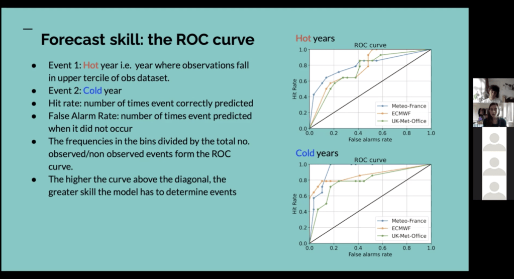
Figure 2: Presenting our project during group project presentations on Friday

Conclusions

The summer school was incredibly smoothly run, very engaging to people both new and experienced in the topic and provided plenty of opportunity to ask questions to the enthusiastic lecturers. Would recommend to PhD students working with forecasts and wanting to assess them!