Deploying an Instrument to the Reading University Atmospheric Observatory 

Caleb Miller – c.s.miller@pgr.reading.ac.uk 

In the Reading area, December and January seem to be prime fog season. Since I’m studying the effects of fog on atmospheric electricity, that means that winter is data collection season! However, in order to begin collecting data in the first year of my PhD, there was only a short amount of time to prepare an instrument and deploy it to the observatory before Christmas. 

One of the instruments that I am using to measure fog is called the Optical Cloud Sensor (OCS). It was designed by Giles Harrison and Keri Nicoll, and it is described in more detail in this paper: (Harrison and Nicoll 2014). The OCS has four channels of LEDs which shine light into the surrounding air. When fog is present, the fog droplets scatter light back to the instrument, where the intensity from each channel can be measured. 

Powering the instrument 

The OCS was originally designed to be flown on a weather balloon, which meant that it was meant to be powered by battery and run for only short periods of time. In my case, however, I wanted the device to be able to continuously collect data over a period of weeks or months without interruption. Then, we would be able to catch any fog events, even if they hadn’t been forecasted. That meant the device would need to be powered by the +15V power supply available at the observatory, and my first step was to create a power adapter for the OCS so that this would be possible. 

Initially, I had been considering using an Arduino microcontroller as a datalogger, so I decided to put together a power adapter on an Arduino shield (a small electronic platform) for maximum convenience. I included multiple voltage levels on my power adapter and connected them to different power inputs on the OCS. Once this was completed, the entire system could now be powered with a single power supply that was available at the observatory! 

I was able to find all of the required parts for the power supply in stock in the laboratory in the Meteorology Department, and I soldered it together in a few days. The technical staff of the university were very helpful in this process! A photograph of the power adapter connected to an Arduino is shown in Figure 1. 

Figure 1. The power adapter for the optical cloud sensor, built on an Arduino shield 

Storing data from the instrument 

Once the power supply had been created, the next step was setting up a datalogging system. On a balloon, the data would be streamed in real-time down to a ground station by radio link. But when this system was deployed to the ground, that would no longer be necessary. 

Instead, I decided to use a CR1000X datalogger from Campbell Scientific. This system has a number of voltage inputs which can be programmed using a graphical interface over a USB connection, and it has a port for an SD card. I programmed the datalogger to sample each of the four analog channels coming from the OCS every five seconds and to store the measurements on an SD card. Collecting the measurements was then as simple as removing the SD card from the datalogger and copying the data to my laptop. This could be done without interrupting the datalogger, as it has its own internal storage, and it would continue measuring while the SD card was removed. 

I had also considered simultaneously logging a digital form of the measurements to an Arduino in addition to the analog measurements made by the datalogger. This would give us two redundant logging systems which would decrease the chances of losing valuable information in the event of an instrument malfunction. However, due to a shortage of time and a technical issue with the instrument’s digital channels, I was unable to prepare the Arduino logger by the time we were ready to deploy the OCS, so we used only the analog datalogger. 

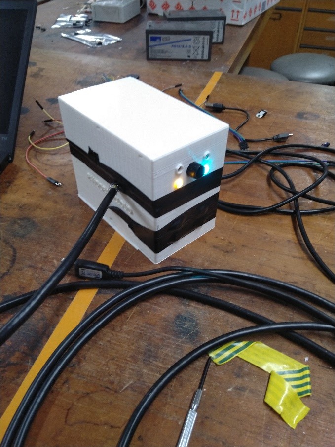
Figure 2. The OCS with its new power supply being tested in the laboratory 

Deploying the instrument 

Once the power supply and datalogger were completed, the instrument was ready to be deployed! It was a fairly simple process to get approval to put the instrument in the observatory; then I met with Ian Read to find a suitable location to set up the OCS. There were several posts in the observatory which were free, and I chose one which was close to the temperature and humidity sensors in the hopes that the conditions would be fairly similar in those locations. Once everything was ready, the technicians and I took the OCS and datalogger and set it up in the field site. At first, when we powered it on, nothing happened. Apparently, one of the solder joints on my power adapter had been damaged when I carried it across campus. However, I resoldered that connection with advice from the university technical staff, and it worked beautifully! 

Figure 3. The datalogger inside its enclosure in the observatory 

Figure 4. The OCS attached to its post in the observatory  

Except for a short period of maintenance in January, the OCS has been running continuously from December until May, and it has already captured quite a few fog events! With the data from the OCS, I now have an additional resource to use in analyzing fog. The levels of light backscattered from the four channels of the instrument provide interesting information, which I am combining with electrical and visibility measurements to analyze the microphysical properties of fog development. 

Hopefully, over the next year, we will be able to measure many more fog events with this instrument that will help us to better understand fog! 

Harrison, R. G., and K. A. Nicoll, 2014: Note: Active optical detection of cloud from a balloon platform. Rev. Sci. Instrum., 85, 066104, https://doi.org/10.1063/1.4882318. 

A new, explicit thunderstorm electrification scheme for the Met Office Unified Model

Email: Benjamin.Courtier@pgr.reading.ac.uk

Forecasting lightning is a difficult problem due to the complexity of the lightning process and how dependent the lightning forecast is on the accuracy of the convective forecast. In order to verify forecasts of lightning independently of the accuracy of the convective forecast, it can be helpful to introduce a lightning scheme that is more complex and physically representative than the simple lightning parameterisations often used in Numerical Weather Prediction (NWP).

The existing method of predicting lightning in the Met Office’s Unified Model (MetUM) uses upwards graupel flux and total ice water path, based on the method of McCaul et al. (2009). However, this method tends to overpredict the total number and coverage of lighting, particularly in the UK.

I’ve implemented a physically based, explicit electrification scheme in the MetUM in order to try and improve the current lightning forecasts. The processes involved in the scheme are shown in the flowchart in Figure 1. The electrification scheme uses the Non-Inductive Charging (NIC) process to separate charge within thunderstorms (Mansell et al., 2005; Saunders and Peck, 1998). The NIC theory states that when graupel and ice crystals collide some charge is transferred from one particle to the other. The sign and the magnitude of the charge that is transferred to the graupel particle depends on a number of parameters. It is affected by the ice crystal diameter, the velocity of the collision, the liquid water content and the temperature at which the collision occurs. Once the charge has been generated on graupel and ice or snow particles, it can be moved around the model domain and can be transferred between hydrometeor species. Charge is removed from hydrometeor species and the domain when the hydrometeors precipitate to the surface or if the hydrometeor evaporates or sublimates. Charge is transferred between hydrometeor species proportionally to the mass that is transferred. Charge is held on graupel, rain and cloud ice (or aggregates and crystals if these are included separately).

Figure 1: A flowchart showing the process and order of those processes involved within the new electrification scheme.

Once these charged hydrometeors are distributed through the cloud, they can be totalled to create a charge density distribution. From this distribution the electric field can be calculated. Then from the electric field lightning flashes can be discharged. Lightning flashes are discharged based on two thresholds, the first of these is the initiation threshold and governs where the initiation point for the lightning channel should be (Marshall et al., 1995). The second of these is a propagation threshold and governs whether or not the lightning channel can move through a grid box (Barthe et al., 2012). Lightning channels are only allowed to propagate vertically within a grid column to simplify the model structure (Fierro et al., 2013). Once the channel is created charge is neutralised along the channel, charge is removed from hydrometeor species in both the channel and the grid points immediately adjacent to the channel.

The updated charge density distribution is then used to recalculate the electric field and new flashes are discharged from any points that exceed the electric field threshold. This process keeps repeating until no new lightning flashes are discharged within the domain.

The plots in Figure 2 show the charge on graupel (a), cloud ice (b), rain (c) and the total charge (d) for a small single cell thunderstorm in the south of the UK on the 31st August 2017. It can be seen in these figure that the charge is mainly positive on cloud ice and mainly negative on graupel. The cloud ice, being less dense is lofted towards the top of the thunderstorm, while the graupel being denser generally falls towards the bottom of the storm. This creates the charge structure seen in Fig. 2d, with two positive-negative dipoles. This charge structure allows for the development of strong electric fields between the positive and negative charge centres in each dipole. If the electric field between the charge centres reaches the order of 100s kVm-1 the air can become electrically conductive, causing lightning.

Figure 2: The charge on hydrometeors in a small single-cell thunderstorm (a) shows the charge on graupel, (b) shows the charge on cloud ice, (c) shows the charge on rain and (d) shows total charge. In each plot, the outline indicated by the solid black line is the 5 dBZ reflectivity contour.

The electrification scheme was run within the operational configuration of the MetUM for a case study. The case study was a case of some organised and some single-cell, fair weather convection, on the 31st August 2017. The observations of lightning flashes are taken from the Met Office’s ATDNet lightning location system. The results of the total lighting accumulated for the entire day of the 31st August are shown in Figure 3. It can be easily seen that the existing method is producing far too much lightning compared to the observations. The new scheme is much closer to the observations.

It is an improvement, not only in the total lightning output, but also in the appearance of the lightning flash map. The scattered nature of the observations is captured by the new scheme, whereas the existing parameterisation appears to be largely producing lightning in neat, contoured paths. These paths show that the way that the existing parameterisation predicts lightning is not physically accurate and indicate the problem with the parameterisation, namely that it relies too heavily on the total ice water path. The new scheme suggests a possible improvement, in considering more explicitly the combination of graupel, liquid water and cloud ice that is vital for the production of charge and therefore lightning.

Figure 3: The total lightning flash accumulation for 31st August 2017 across the UK, (a) shows the output of the new electrification scheme, (b) shows the observed flashes, binned to match the model grid, and (c) shows the output of the existing MetUM parameterisation.

References:
Barthe, C., Chong, M., Pinty, J.-P., and Escobar, J. (2012). CELLS v1.0: updated and parallelized version of an electrical scheme to simulate multiple electrified clouds and flashes over large domains. Geoscientific Model Development, (5), 167–184.

Fierro, A. O., Mansell, E. R., MacGorman, D. R., and Ziegler, C. L. (2013). The Implementation of an Explicit Charging and Discharge Lightning Scheme within the WRF-ARW Model: Benchmark Simulations of a Continental Squall Line, a Tropical Cyclone, and a Winter Storm. Monthly Weather Review, 141, 2390–2415.

Mansell, E. R., MacGorman, D. R., Ziegler, C. L., and Straka, J. M. (2005). Charge structure and lightning sensitivity in a simulated multicell thunderstorm. Journal of Geophysical Research, 110.

Marshall, T. C., McCarthy, M. P., and Rust, W. D. (1995). Electric field magnitudes and lightning initiation in thunderstorms. Journal of Geophysical Research, 100, 7097–7103.

McCaul, E. W., Goodman, S. J., LaCasse, K. M., and Cecil, D. J. (2009). Forecasting lightning threat using cloud-resolving model simulations. Weather and Forecasting, 24(3), 709–729.

Saunders, C. P. R. and Peck, S. L. (1998). Laboratory studies of the influence of the rime accretion rate on charge transfer during crystal / graupel collisions. Journal of Geophysical Research, 103, 949–13.