Anyone that has ever been on a plane will probably have experienced turbulence at some point. Most of the time it is not likely to cause injury, but during severe turbulence unsecured objects (including people) can be thrown around the cabin, costing the airline industry millions of dollars every year in compensation (Sharman and Lane, 2016). Recent research has also indicated that in the future the frequency of clear-air turbulence will increase with climate change. Forecasting turbulence is one of the best ways to reduce the number of injuries by giving pilots and flight planners ample warning, so they can put on the seat-belt sign or avoid the turbulent region altogether. The current method used in creating a turbulence forecast is a single ‘deterministic’ forecast – one forecast model, with one forecast output. This shows the region where they suspect turbulence to be, but because the forecast is not perfect, it would be more ideal to show how certain we are that there is turbulence in that region.
To do this, a probabilistic forecast can be created using an ensemble (a collection of forecast model outputs with slightly different model physics or initial conditions). A probabilistic forecast essentially shows model confidence in the forecast, and therefore how likely it is that there will be turbulence in a given region. For example, if all 10 out of 10 forecast outputs predict turbulence in the same location, the pilots would be confident in taking action (such as avoiding the region altogether). However, if only 1 out of 10 models predict turbulence, then the pilot may choose to turn on the seat-belt sign because there is still a chance of turbulence, but not enough to warrant spending time and fuel to fly around the region. A probabilistic forecast not only provides more information in the certainty of the forecast, but it also increases the chances of forecasting turbulence that a single model might miss.
Gill and Buchanan (2014) showed this ensemble forecast method does improve the forecast skill. In my project we have taken this one step further and created a multi-model ensemble, which is combining two different ensembles, each with their own strengths and weaknesses (Storer et al., 2018). We combine the Met Office Global and Regional Ensemble Prediction System (MOGREPS-G), with the European Centre for Medium Range Weather Forecasting (ECMWF) Ensemble Prediction System (EPS).

There are three main sources of turbulence. The first is mountain wave turbulence, where gravity waves are produced from mountains that ultimately lead to turbulence. The second is convectively-induced turbulence, which includes in-cloud turbulence and also gravity waves produced as a result of deep convection that also lead to turbulence. The third is shear-induced turbulence, which is the one we are trying to forecast in this example. Figure 1 is an example plot showing orography and thus mountain wave turbulence (top left), convection and thus convectively induced turbulence (top right), the MOGREPS-G ensemble forecast of shear turbulence (bottom left) and the ECMWF ensemble forecast of shear turbulence (bottom right). The red circle indicates a ‘moderate or greater’ turbulence event, and we can see that because it is over the North Atlantic it is not a mountain wave turbulence event, and there is no convection nearby, but both the ensemble forecasts correctly predict the location of the shear-induced turbulence. This shows that there is high confidence in the forecast, and action (such as putting the seat-belt sign on) can be taken.
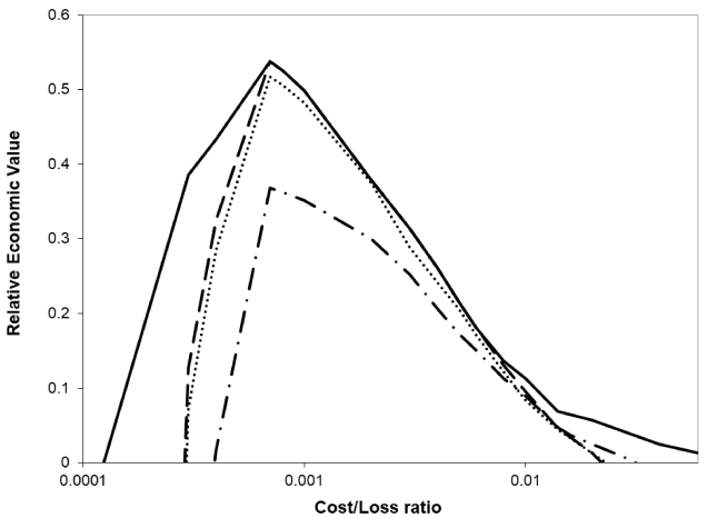
To understand the usefulness of the forecast, Figure 2 is a relative economic value plot. It shows the value of the forecast for a given cost/loss ratio (which will vary depending on the end user). The multi-model ensemble is more valuable than both of the single model ensembles for all cost/loss ratios, showing that every end user will benefit from this forecast. Although our results do show an improvement in forecast skill, it is not statistically significant. However, by combining ensemble forecasts we gain consistency and more operational resilience (i.e., we are still able to produce a forecast if one ensemble is not available), and is therefore still worth implementing in the future.
Email: luke.storer@pgr.reading.ac.uk
References
Gill PG, Buchanan P. 2014. An ensemble based turbulence forecasting system. Meteorol. Appl. 21(1): 12–19.
Sharman R, Lane T. 2016. Aviation Turbulence: Processes, Detection, Prediction. Springer.
Storer, L.N., Gill, P.G. and Williams, P.D., 2018. Multi-Model Ensemble Predictions of Aviation Turbulence. Meteorol. Appl., (Accepted for publication).
