By Elliot Mckinnon-Gray and Niamh Ocallaghan
The making of 2024’s departmental pantomime Stratatouille actually began all the way back in the summer of that year. There had been conversations on some stifling hot days (not that there were many!) around the theme for the current year’s panto. A film viewing had taken place and characters had begun to be assigned. However, come October, no one could have predicted the twist this tale would have taken leading to the majority of PhD students reluctantly(?) donning chef hats and rat ears for the best part of the coming December.

STRATATOUILLE Poster
Our story actually begins even earlier, mere days after the roaring success of sshRACC in December 2023 – as is apparently tradition – the fabled Panto Cupboard Key was foisted upon me by one of last year’s organisers. I won’t name and shame – but my fate was sealed; I was to become the organiser for the 2024 departmental pantomime. But who, pray, would heed my call for a co-organiser in this, my hour of need? It all came down to a rather conniving bit of deception, whereby I managed to trick my co-coordinator into accepting the key when they may have been expecting a tasty treat. Who says the pantomime is begrudgingly organised? But our destiny was well and truly decided and laid out in front of us. In nine to ten short months, we would be organising a corral of unruly PhD students and support staff to put on the world’s greatest annual university meteorology department pantomime.
Coming back to where we began, at the start of the academic year, we had an extremely strong candidate for what we thought was going to be the theme of the panto, but as always, the story for the panto is decided in the second(?) PhD Group Meeting of the year in a democratic process. This is where our original plan got unseated. The strongest proprietor (with many supporters) of the originally planned theme made the fatal mistake of prioritising career development over their wishes for a panto theme and could not make the deciding session. As Rabbie Burns reminds us, “The best laid plans of mice and men often go awry” – this was one such instance. With only half the organising committee present to propose the original idea, a plucky upstart with one good joke took the stage and captured the imagination of the PhD cohort, and so it was decided: Stratatouille would be the theme for this year’s panto. As fatefully predicted in last year’s panto blog post…
Plot
After innumerable lunchtime and evening writing sessions, the bulk of the panto story was baked and ready to consume. It is here where we have to give another massive thank you to Caleb Miller, who spent hours and hours essentially transposing the original story of the film Ratatouille to be based in our department following the terribly cobbled together idea of a story that we had. All we had to do now was pepper it with jokes and puns pertaining to food and/or meteorology and we had a script that even Patton Oswalt would be proud to perform.
Audience review #1
“The best panto I’ve seen for many years”
– Dr. Pete Inness
The story begins with Remi the undergrat realising he feels unable to fulfil his ambition of doing serious research while surrounded by his decidedly unserious fellow undergrats. All they care about is getting drunk off snakebites, but Remi has a dream of becoming a great scientist and doing exceptional and interesting original research. While feeling dejected that he is too inferior to publish original research, he has an apparition of King Sir Professor Brian Hoskins* who gives him a message that anyone can be a scientist if they put their heart into it.
Then we meet Linguini, a floundering PhD student who feels like he isn’t cut out for the work he is undertaking and expected to do. In a moment of serendipity, Linguini leaves his laptop open and unlocked in the BH coffee area where Remi is able to take a look at the work he is carrying out analysing some CheeseCDF files. Remi realises Linguini’s coding is terrible, fixes a few bugs and manages to greatly improve the code Linguini was working on. This leads to Linguini accepting help from Remi to write a paper as part of his PhD.
In the next scene, Linguini is showing Remi around his PhD office, when the WCD (Weekly Cuisine Discussion) bell goes, and all the PhD students diligently trudge down to GU01 to attend. Admittedly the WCD scene doesn’t further the story much apart from giving Remi an insight into the breadth of research done in this meteorology kitchen. But we got a lot of laughs, good jokes and puns, and silly costumes into this scene so it was an audience and cast favourite. It is later in this scene that we meet the terrifying supervisor, brilliantly played by our regular cartoon villain Catherine Toolan. The supervisor is very tough on Linguini with high expectations and little patience. But that is all too easy for Remi who manages to complete the task the supervisor asked for in no time at all. They (Linguini napping with his feet up) spend the next few hours “cooking up some actual research”. When the supervisor returns, she is amazed to see that ‘Linguini’ has disproved the entire concept of PV. Suspicious that he has managed to attain such a level of skill so quickly, she recommends that he first present the work at a conference before they crack on with publishing the work.
At the conference, Linguini gives a great presentation (Remi is giving him slide-by-slide instructions) but makes a fatal error by taking nearly all of the credit and failing to mention he got any help from Remi. This alienates Remi who storms out of the conference to return to the department. Jumping forward in time, when Remi returns to and hatches a cunning plan to derail the entire department – stealing the tea and coffee money box (topical departmental news has appeared in the script!). Back at the conference, Remi is making a total fool of himself by not being able to answer even the simplest of questions from the audience, embarrassing his supervisor in the process. She interrogates him about this and finds out much to her dismay that an undergrat helped with the research. So disgusted is she at this that supervisor and the other staff members strike, leaving the department destitute of senior figures.
This leads to a moment where Remi and Linguini make up thanks to an apology, and Remi recruits a team of undergrats to help finish writing the paper they started. The paper is submitted to the journal Nature: Valley Bar where it is eventually inspected by the feared Reviewer 2, who is so impressed by the work that he recommends it be published with no changes (apart from citing one of his own papers). The story ends with KSPBH* re-appearing and handing Remi the keys to the department and naming the building after him.
Songs
Please Stop Me Now – there was a running theme of ‘difficult to sing but possibly worth the effort since they are well loved tunes’ for most songs this year, and this one was no exception. A parody of Queen’s 1979 mega-hit of Don’t Stop Me Now, our extremely talented band carried our pretty rubbish singing – but that didn’t stop it being some attendees’ favourite part of the show.
Audience review #2
“How did you guys come up with all those song lyrics and make them work? So funny and so impressive!”
– MSc Student
Come on Remi – One of the more singable tunes based on Come on Eileen by Dexys Midnight Runners, all about how much work Remi was going to have to do to get Linguini through his PhD work. In practising this one, we had choir master Catherine bellowing at us to sing louder, a task we all found much easier after a few glasses of boxed wine from the Winnersh Sainsbury’s. The Middle – Jimmy Eat World was the third song which I don’t think we even came up with a spoof title for; a punk-pop particularly catchy tune about the trials and tribulations of poor Linguini the PhD first year who is letting his stress get in the way of enjoying the start of his PhD. Money, Money, Money – an ABBA classic we also didn’t need to change the title of about the rats stealing the money box. We made the bold decision this year to plant much of the songs mid-scene. A directorial choice that I think helped the coherent telling of the story. Special mention here to Nathan’s amazing piano playing skills here – the rendition of Erik Satie’s Gymnopedie during the John Meth-Coq-au-Vin monologue was only improvised in the final dress rehearsal earlier that day! 500 Lines – a version of the Proclaimers’ singalong classic 500 Miles about how many lines Remi has to write to get their paper done! H-O-S-K-I-N-S : I’m not sure how Sir Brian feels about being the subject of the panto or at least a song every year, and this one was a little on the nose; but you really couldn’t ask for a better fit for one of the songs of the summer – Chappell Roan’s Hot to Go had exactly the right mood for what we wanted to sing, and I think it made for a great outro wonderfully delivered by one of the best KSPBH performances we’ve seen in a while by our very own Douglas Mulangwa.
Casting
It can be a bit like pulling teeth trying to cast the leading roles in the panto, and as one of the few first-year PhDs who have shown the extroversion to be able to tackle this and with great stage presence, the inimitable Jake Keller somewhat reluctantly agreed to be Remi with a fateful “if I have to” when asked repeatedly. I think he came around to really enjoying it, and the audience were also quite impressed –
Audience review #3
[To Jake] “You were great!”
– Regius Professor Keith Shine
And Andrea Rivosecchi as Linguini – at first he accepted but then realised he would have to learn even more lines than the main character; so we looked around and found a great doppelganger for the second act – not sure if any of you noticed – but in the second act Linguini was played by a different Italian man in Riccardo Monfardini! Some veterans of the game came through and gave us some great performances with Catherine as Supervisor and Hette Houtman as Pete Dinners. Shout out to Hette as one of last year’s organisers for also helping us with timing and who to contact for various admin duties. The remaining roles had under 5 lines, but all were delivered hilariously and brilliantly, and you all appear to have agreed.
Audience Review #5
“Catherine was quite scary as supervisor”
– Dr Andy Apple Turnover Turner (Catherine’s PhD Supervisor)
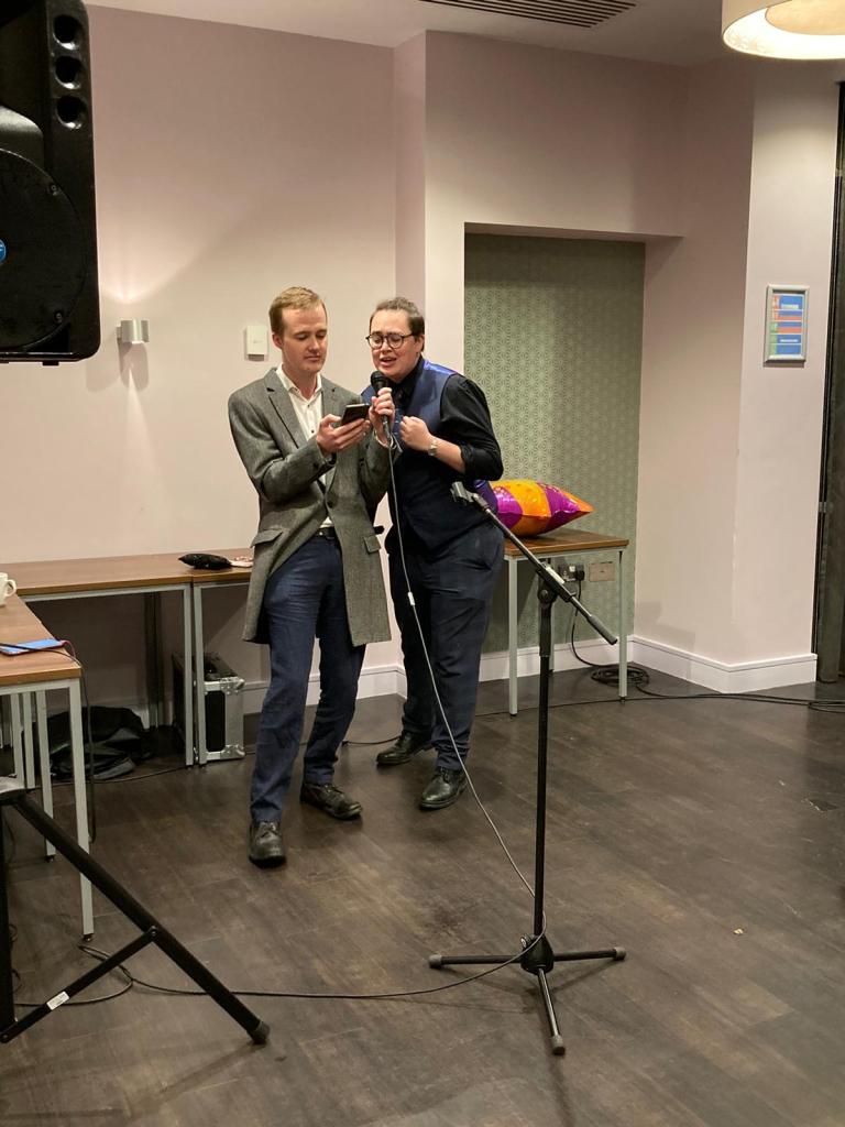
The Night (and Day) of the Panto
So as many of you agreed, the Act 1 cameo from our antipodean friend Robbie Marks (the star of last year’s panto) was one of the best moment’s of the panto:
Audience review #4
“I can’t believe Robby came through and made that for us!”
– Gabrielle Ching-Johnson (Undergrat #2)
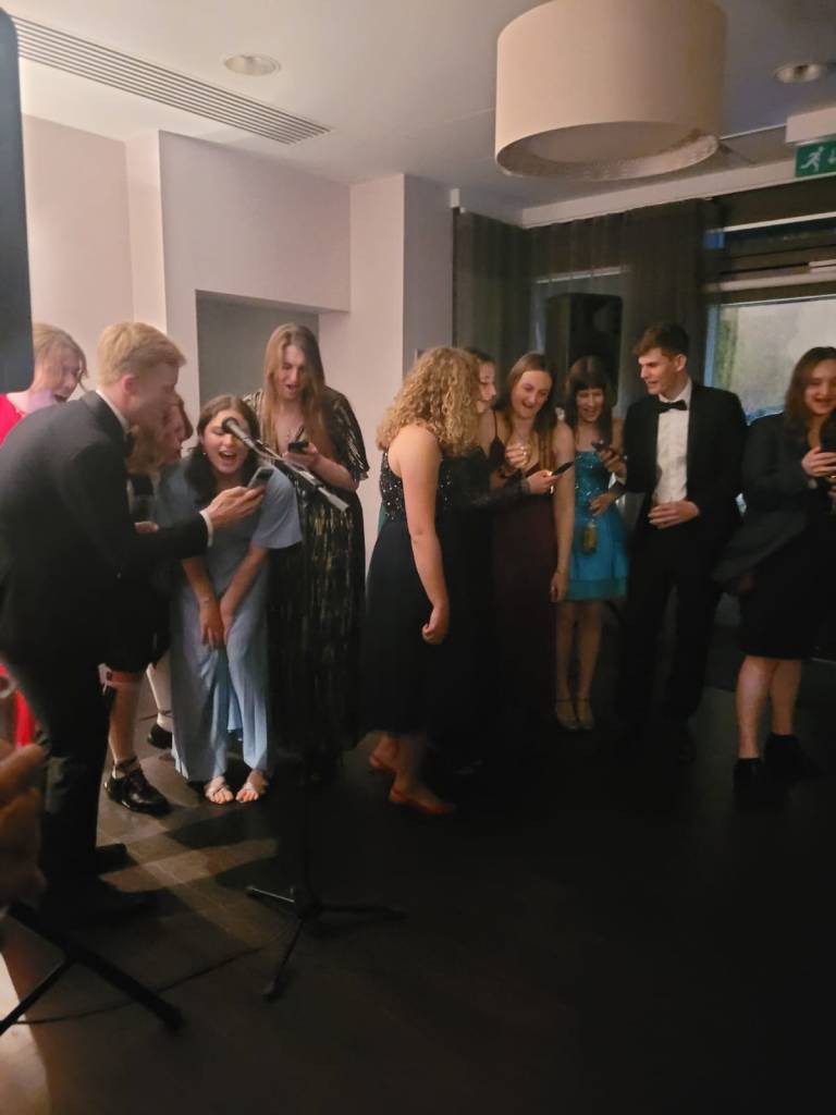
This is where I would like to make the point that he sent me those videos the morning of the show, and we had to hurriedly stitch together his several renditions of that speech in different locations with the cinematic walk off. Special thanks to Rosie (last year’s co-organiser) for helping with the video editing, and generally for being a great help to us organisers this year by giving advice and keeping us on time (mostly). Robby was sent a video of the mirthful reaction to his cameo with the reaction “F*** yeah, glad I could make an appearance”. The day went much more smoothly than last year, with us occupying the Madejski lecture theatre from 2pm onwards with no interruptions, we had plenty of time to set up the tech and instruments, as well as squeeze in a final full rehearsal. Set up the ticket booth, and we were ready to go! 150 people filed in for a great attendance to our show. Not to forget a great buffet beforehand to get everyone in the mood for the flagship event in the departmental calendar.
Act 1 and Act 2 managed to run for about the same amount of time, 30 mins a piece for an hour-long panto, as we had planned – brilliant! The interval acts, however put paid to that. A mammoth 45-minute session full of controversy and some of the biggest laughs of the night. We saw Stroopwaffels crowned the winner of the big biscuit bracket, however this was vetoed by the head of department who quite rightly pointed out they are not a biscuit and so the runner up chocolate hobnobs was our true champion. Professor Coq-au-Vin was not the only one to take issue with this controversial result. The 3L68 team of Dan Shipley, Jake Bland and Brian Lo made the argument that Bourbons had been wrongfully expelled and would have won this year, and so Dan delivered a hilarious diatribe explaining how they came to decide which Bourbon was best, and therefore the true winner of the biscuit bracket. I don’t remember which one it was in the end (M&S?) – check the video recordings of the night to find out for yourselves.
A pleasant break from the commotion of the biscuit brackets was brought around from some classical piano performed by Amber Te Winkel, and then some might say the only reason they attend the panto – Mr Mets. A blinder of an episode where Peter Clark was apologised to (again – and rejected on his behalf by Humphrey), and insinuated to have signed up to OnlyFans with the most innocent of intentions. The theme of the story was John Methven’s takeover as head of department, with him bumbling along and struggling to fulfil the role while eating copious amounts of ‘free’ food (it’s not free if you use department funds to pay for it, Prof. Methven!). Just to clarify that no one thinks John will struggle to fulfil the role, but as HOD I’m afraid you have to expect a fair bit of derision at these sorts of performances!
Following that, another side-splittingly funny act followed with an after party led by DJ Shonk that included a rare slow number – all in aid of blossoming romance on the dancefloor.
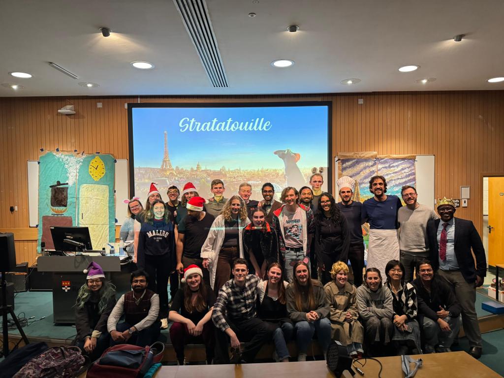
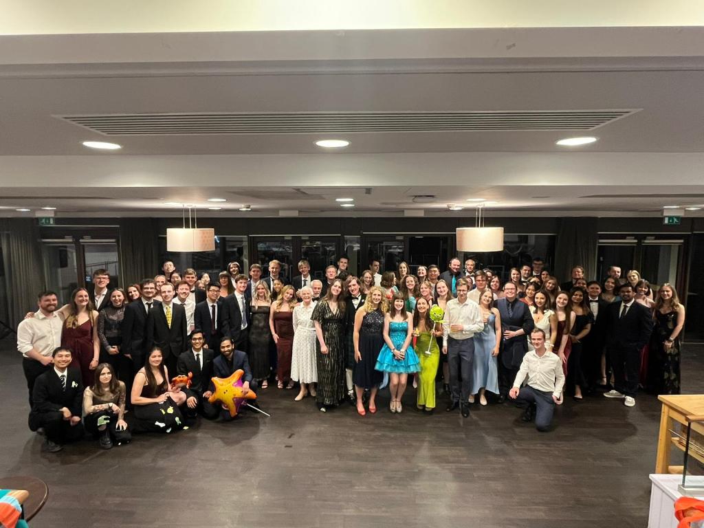
The amazing cast and crew who made STRATATOUILLE happen!
Reflections
As always, the Panto is months of hard work to organise, and things only ever seem to come together in the eleventh hour. But we had a great team and cast and band that really made it come together beautifully. Acting on stage, playing in a live band, organising a production, generally being a thesp isn’t the kind of thing you expect to hear from a large majority of the PhD students of the world’s leading Meteorology department. But it is these experiences, very far outside most of our comfort zones that builds strong and adaptable characters. And I think this experience has probably given us, as organisers and performers alike, more useful skills than we might have realised. This will, however, probably be these director-producers’ debut and final production.
A huge thank you to everyone who attended and contributed to the panto in any way, no matter how small. Your participation is what makes this a great bonding experience for the department, and you are all greatly appreciated!
One last time,
Your Panto Organisers
Elliot and Niamh