You may have heard the term Tiger Teams mentioned around the department by some PhD students, in a SCENARIO DTP weekly update email or even in the department’s pantomime. But what exactly is a tiger team? It is believed the term was coined in a 1964 Aerospace Reliability and Maintainability Conference paper to describe “a team of undomesticated and uninhibited technical specialists, selected for their experience, energy, and imagination, and assigned to track down relentlessly every possible source of failure in a spacecraft subsystem or simulation”.
This sounds like a perfect team activity for a group of PhD students, although our project had less to do with hunting for flaws in spacecraft subsystems or simulations. Translating the original definition of a tiger team into the SCENARIO DTP activity, “Tiger Teams” is an opportunity for teams of PhD students to apply our skills to real-world challenges supplied by industrial partners.
The project culminated in a visit to the Met Office to present our work.
Why did we sign up to Tiger Teams?
In addition to a convincing pitch by our SCENARIO director, we thought that collaborating on a project in an unfamiliar area would be a great way to learn new skills from each other. The cross pollination of ideas and methods would not just be beneficial for our project, it may even help us with our individual PhD work.
More generally, Tiger Teams was an opportunity to do something slightly different connected to research. Brainstorming ideas together for a specific real-life problem, maintaining a code repository as a group and giving team presentations were not the average experiences one could have as a PhD student. Even when, by chance, we get to collaborate with others, is it ever that different to our PhD? The sight of the same problems …. in the same area of work …everyday …. for months on end, can certainly get tiring. Dedicating one day per week on an unrelated, short-term project which will be completed within a few months helps to break the monotony of the mid-stage PhD blues. This is also much more indicative of how research is conducted in industry, where problems are solved collaboratively, and researchers with different talents are involved in multiple projects at once.
What did we do in this round’s Tiger Teams?
One project was offered for this round of Tiger Teams: “Crowdsourced Data for Machine Learning Prediction of Urban Heat Wave Temperatures”. The bones of this project started during a machine learning hackathon at the Met Office and was later turned into a Tiger Teams proposal. Essentially, this project aimed to develop a machine learning model which would use amateur observations from the Met Offices Weather Observation Website (WOW), combined with landcover data, to fine-tune model outputs onto higher resolution grids.
Having various backgrounds from environmental science, meteorology, physics and computer science, we were well equipped to carry out tasks formulated to predict urban heat wave temperatures. Some of the main components included:
Quality control of data – as well as being more spatially dense, amateur observation stations are also more unreliable
Feature selection – which inputs should we select to develop our ML models
Error estimation and visualisation – How do we best assess and visualise the model performance
Spatial predictions – Developing the tools to turn numerical weather prediction model outputs and high resolution landcover data into spatial temperature maps.
Our supervisor for the project, Lewis Blunn, also provided many of the core ingredients to get this project to work, from retrieving and processing NWP data for our models, to developing a novel method for quantifying upstream land cover to be included in our machine learning models.
An example of the spatial maps which our ML models can generate. Some key features of London are clearly visible, including the Thames and both Heathrow runways.
What were the deliverables?
For most projects in industry, the team agrees with the customer (the industrial partner) on end-products to be produced before the conclusion of the project. Our two main deliverables were to (i) develop machine learning models that would predict urban heatwave temperatures across London and (ii) a presentation on our findings at the Met Office headquarters.
By the end of the project, we had achieved both deliverables. Not only was our seminar at the Met Office attended by more than 120 staff, we also exchanged ideas with scientists from the Informatics Lab and briefly toured around the Met Office HQ and its operational centre. The models we developed as a team are in a shared Git repository, although we admit that we could still add a little more documentation for future development.
As a bonus deliverable, our supervisor (and us) are consolidating our findings into a publishable paper. This is certainly a good deal considering our team effort in the past few months. Stay tuned for results from our paper perhaps in a future blog post!
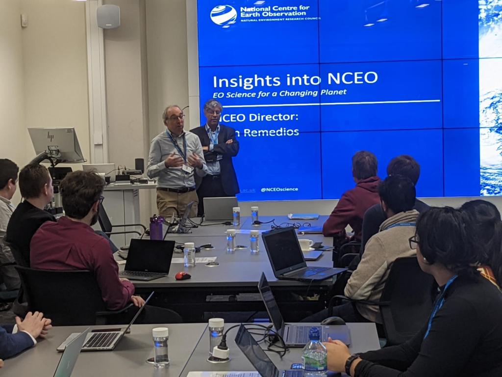
The National Centre for Earth Observation (NCEO) is a distributed NERC centre of over 100 scientists from UK universities and research organisations (https://www.nceo.ac.uk). Last month NCEO launched a new and exciting headquarters, the Leicester Space Park. After the launch, researchers from various institutions with affiliations to NCEO were invited to a forum at the new HQ. This was an introductory workshop in Machine Learning and Artificial Intelligence. We were both lucky enough to attend this in-person event (with the exception of a few remote speakers)!
As first year PhD students, we should probably introduce ourselves:
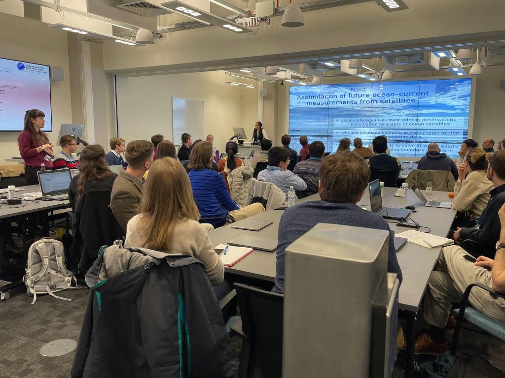
Laura – I am a Scenario student based in the Mathematics department, my project is ‘Assimilation of future ocean-current measurements from satellites’. This will involve applying data assimilation to assimilate ocean-current velocities in preparation for data from future satellites. My supervisor is also the training lead and co-director of Data Assimilation at NCEO. I was thrilled to be able to attend this forum to learn new techniques that can be used in earth observation.
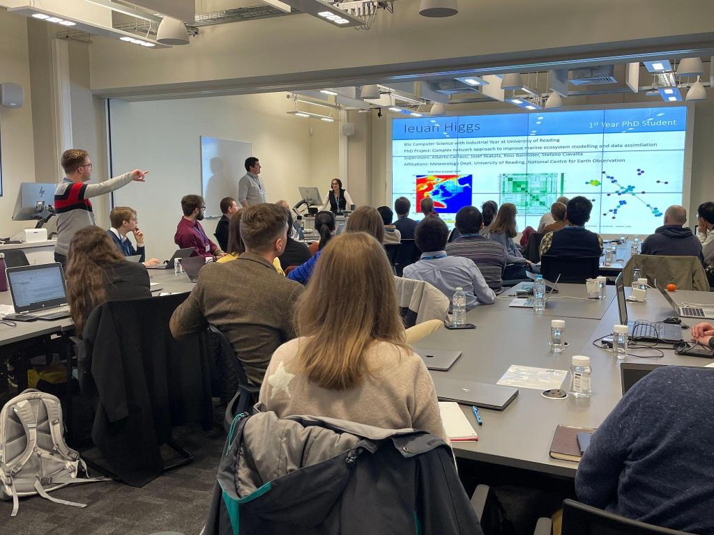
Ieuan – I am a Scenario Associate based in the Meteorology department. My project is titled ‘Complex network approach to improve marine ecosystem modelling and data assimilation’. In my work, I hope to apply some complex-network-informed machine learning techniques to predict concentrations of the less well observable nutrients in the ocean, from the well observable quantities – such as phytoplankton! As a member and fundee of NCEO, I was excited to see a training event on offer that was highly relevant to my project.
Machine Learning (ML) and Artificial Intelligence (AI) are often thought of as intimidating and amorphous topics. This fog of misconceptions was quickly cleared up, however, as the workshop provided a brilliant, fascinating and well-structured introduction into how these fields can be leveraged in the context of earth observation.
Introduction to NCEO
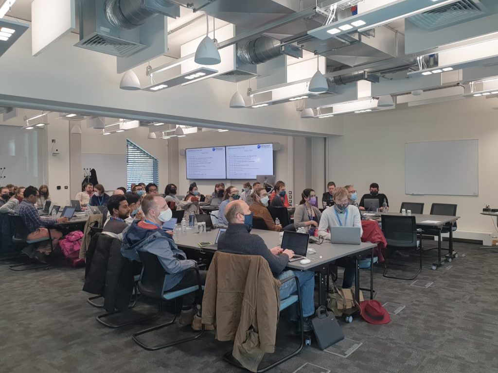
The forum began bright and (very) early on Wednesday morning at the Leicester Space Park. Our first day of ML training began with an introduction to NCEO by director – John Remedios, and training lead – Amos Lawless. We each had the opportunity to introduce ourselves and our research in a quick two-minute presentation. This highlighted the variety in both background and experience in an entirely positive way! As well as benefiting directly from the training itself, we enjoyed being in a room full of enthusiastic people with knowledge and niches aplenty.
Introducing ourselves and our research
Next, we had a talk from Sebastian Hickman, a PhD student at the University of Cambridge, who introduced his work on using ML with satellite imagery to detect tall-tree-mortalities in the Amazonian rainforest. A second talk was given by Duncan Watson-Parris from the University of Oxford on using ML to identify ship tracks from satellite imagery. These initial talks immediately got us thinking about the different ways in which ML could be used within the realm of earth science. The second day we also had talks from ESA’s Φ-lab, on a whole host of different uses for AI in earth observation.
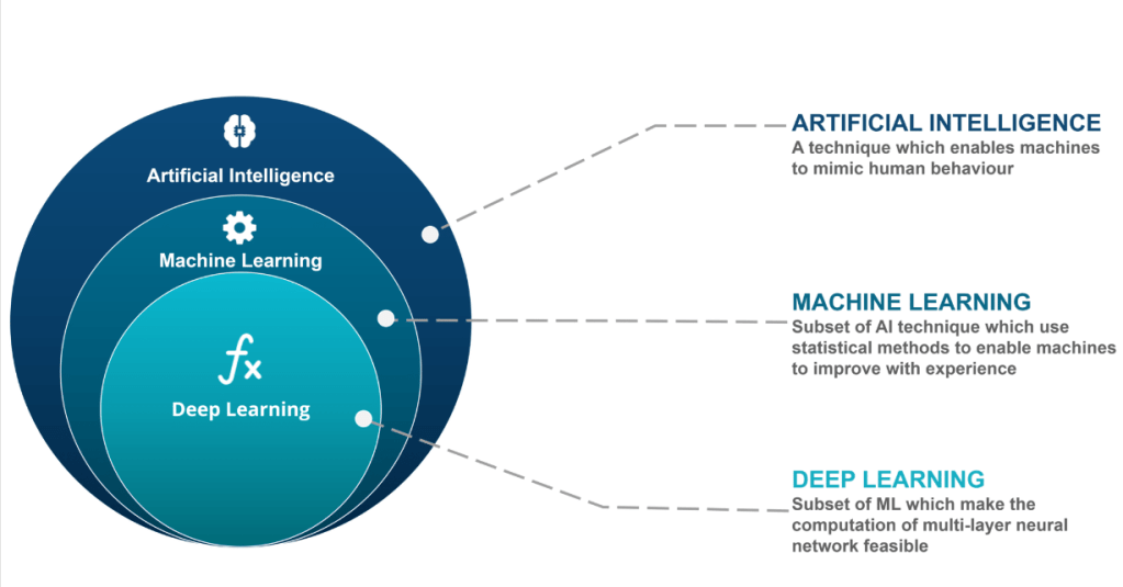
To begin our ML training, members of NEODAAS (NERC Earth Observation Data Acquisition and Analysis Service), David Moffat and Katie Awty-Carroll, led us through an introduction into ML and AI, its uses and importance in modern scientific context. The graphic below – presented by David and Katie – makes a digestible distinction between some commonly conflated terms in the subject area:
AI vs ML vs DL*
The discussion on the limitations and ‘bottlenecks’ of ML was of particular interest, it highlighted the numerous considerations to be made when developing an ML solution. For example, the subset of data used to train a model should ideally be representative of the entire system, avoiding or at least acknowledging the potential biases introduced by: human-preferences in selecting and filtering training data; the method of data collection method; the design of the ML techniques used; and how we interpret the outputs. While this may seem obvious at first, it is certainly not trivial. There are high-profile and hotly-debated examples of AI being used in the real-world where biases have led to significant human-affecting consequences. (https://sitn.hms.harvard.edu/flash/2020/racial-discrimination-in-face-recognition-technology) (https://www.ncbi.nlm.nih.gov/pmc/articles/PMC6875681)
We were prompted to consider these ethical questions and the efficacy of ML in the context of earth science: Which problems does ML help us solve and, perhaps more importantly, which problems are we willing to entrust it with?
A fun exercise you can try for yourself: search for images of a given profession in your search engine of choice. See if you can identify any patterns or biases in what may have been included or even excluded from the selected results!
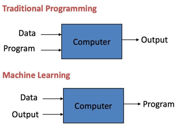
We then began the practical sessions which all fell within the broad umbrella of ML. This required a slight mindset shift from traditional programming as, even from a top-down perspective, the way we approached problems was completely different:
Figure: Traditional Programming vs Machine Learning*
We were given jupyter notebooks to work on three separate practical’s; random forest classification, neural network for regression, and convolutional neural networks. Each showed a different application and use-case of ML, giving us more ideas on how it could potentially be implemented into our own research. Adjacent to this, we were given a workflow task to think about over the two days: how could we use ML in our own projects? At the end of the second day we each presented our ideas and were given feedback. This helped ground the talks with an ongoing focus to relate new knowledge back to our own varied fields; allowing the workshop to elegantly handle the variety and promote the actual use of the skills in our own work.
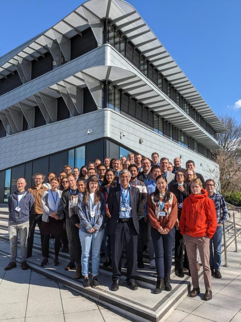
The forum was academically challenging but it was also great fun! Surrounding the concentrated days of learning, the forum offered us plenty of chances to connect with others. We were given a tour of the Space Park, an impressive space you could say was out of this world. The evening activities, bowling and shuffleboard, had a great atmosphere too!
NCEO Forum Delegates 2022 outside Leicester Space Park
By the end of the event, the interest and enthusiasm of the attendees had been effectively transformed into new understanding and conversation – which is unsurprising considering the increasing relevance ML is gaining in the field of earth science. Further to this, making connections over the pandemic has been difficult, so we felt extremely fortunate that we were able to meet in person.
Laura– The forum was an exciting insight into a field I had no experience in. Although my immediate work is focused on the application of data assimilation to ocean measurements, which does not directly relate to ML at the moment, data assimilation has high potential to overlap with ML .The forum has furthered my understanding of fields that surround the focal point of my research. In turn, this has helped me gain a more well-rounded knowledge base, opening doors to new directions my research could take.
Ieuan – The forum has certainly given me many new avenues to explore when approaching the intended application of ML in my work, perhaps starting simple with a neural network for multivariate regression and expanding from there. The hands-on practicals were a valuable opportunity for practice and a great chance for some informal discussion on the details of ML implementation with my peers. Moreover, the event has equipped us with the skills to effectively engage with other academics when they present ML-based work – which is something I would love to do in future events!
We both hope there will be more NCEO workshops like this in the future, perhaps an event or meetup that focuses on the intersection of ML and data assimilation, as these topics resonate with us both. We’d like to thank the NEODAAS staff from PML for leading the training and Uzma Saeed for organising the forum. It was a fun and engaging experience that we are grateful to have taken part in and we would encourage anyone with the opportunity to learn about ML to do so!
* Graphics were provided by the NEODAAS slides used at the NCEO forum
Figure 1 Replica of the first 1643 Torricelli barometer [1]
Humans have tried, for millennia, to predict the weather by finding physical relationships between observed weather events, a notable example being the descent in barometric pressure used as an indicator of an upcoming precipitation event. It should come as no surprise that one of the first weather measuring instrument to be invented was the barometer, by Torricelli (see in Fig. 1 a replica of the first Torricelli barometer), nearly concurrently with a reliable thermometer. Only two hundred years later, the development of the electric telegraph allowed for a nearly instant exchange of weather data, leading to the creation of the first synoptic weather maps in the US, followed by Europe. Synoptic maps allowed amateur and professional meteorologists to look at patterns between weather data in an unprecedented effective way for the time, allowing the American meteorologists Redfield and Epsy to resolve the dispute on which way the air flowed in a hurricane (anticlockwise in the Northern Hemisphere).
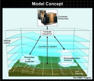
Figure 2 High Resolution NWP – model concept [2]
By the beginning of the 20th century many countries around the globe started to exchange data daily (thanks to the recently laid telegraphic cables) leading to the creation of global synoptic maps, with information in the upper atmosphere provided by radiosondes, aeroplanes, and in the 1930s radars. By then, weather forecasters had developed a large set of experimental and statistical rules on how to compute the changes to daily synoptic weather maps looking at patterns between historical sets of synoptic daily weather maps and recorded meteorological events, but often, prediction of events days in advance remained challenging.
In 1954, a powerful tool became available to humans to objectively compute changes on the synoptic map over time: Numerical Weather Prediction models. NWPs solve numerically the primitive equations, a set of nonlinear partial differential equations that approximate the global atmospheric flow, using as initial conditions a snapshot of the state of the atmosphere, termed analysis, provided by a variety of weather observations. The 1960s, marked by the launch of the first satellites, enabled 5-7 days global NWP forecasts to be performed. Thanks to the work of countless scientists over the past 40 years, global NWP models, running at a scale of about 10km, can now simulate skilfully and reliably synoptic-scale and meso-scale weather patterns, such as high-pressure systems and midlatitude cyclones, with up to 10 days of lead time [3].
The relatively recent adoption of limited-area convection-permitting models (Fig. 2) has made possible even the forecast of local details of weather events. For example, convection-permitting forecasts of midlatitude cyclones can accurately predict small-scale multiple slantwise circulations, the 3-D structure of convection lines, and the peak cyclone surface wind speed [4].
However, physical processes below convection permitting resolution, such as wind gusts, that present an environmental risk to lives and livelihoods, cannot be explicitly resolved, but can be derived from the prognostic fields such as wind speed and pressure. Alternative techniques, such as statistical modelling (Malone model), haven’t yet matched (and are nowhere near to) the power of numerical solvers of physical equations in simulating the dynamics of the atmosphere in the spatio-temporal dimension.
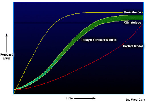
Figure 3 Error growth over time [5]
NWPs are not without flaws, as they are affected by numerical drawbacks: errors in the prognostic atmospheric fields build up through time, as shown in Fig. 3, reaching a comparable forecast error to that of a persisted forecast, i.e. at each time step the forecast is constant, and of a climatology-based forecast, i.e. mean based on historical series of observations/model outputs. Errors build up because NWPs iteratively solve the primitive equations approximating the atmospheric flow (either by finite differences or spectral methods). Sources of these errors are: too coarse model resolution (which leads to incorrect representation of topography), long integration time steps, and small-scale/sub-grid processes which are unresolved by the model physics approximations. Errors in parametrisations of small-scale physical processes grow over time, leading to significant deterioration of the forecast quality after 48h. Therefore, high-fidelity parametrisations of unresolved physical processes are critical for an accurate simulation of all types of weather events.
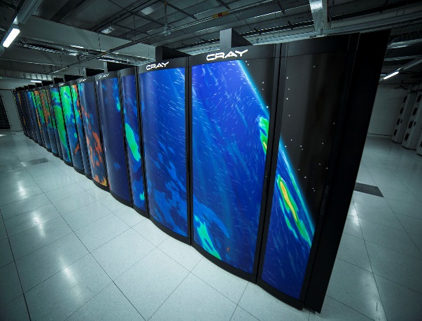
Figure 4 Met Office HPC [6]
Another limitation of NWPs is the difficulty in simulating the chaotic nature of weather, which leads to errors in model initial conditions and model physics approximations that grow exponentially over time. All these limitations, combined with instability of the atmosphere at the lower and upper bound, make the forecast of rapidly developing events such as flash floods particularly challenging to predict. A further weakness of NWP forecasts is that they rely on the use of an expensive High Parallel Computing (HPC) facility (Fig. 4), owned by a handful of industrialised nations, which run coarse scale global models and high-resolution convection-permitting forecasts on domains covering area of corresponding national interest. As a result, a high resolution prediction of weather hazards, and climatological analysis remains off-limits for the vast majority of developing and third-world countries, with detrimental effects not just on first line response to weather hazards, but also for the development of economic activities such agriculture, fishing, and renewable energies in a warming climate. In the last decade, the cloud computing technological revolution led to a tremendous increase in the availability and shareability of weather data sets, which transitioned from local storage and processing to network-based services managed by large cloud computing companies, such as Amazon, Microsoft or Google, through their distributed infrastructure.
Combined with the wide availability of their cloud computing facilities, the access to weather data has become more and more democratic and ubiquitous, and consistently less dependent on HPC facilities owned by National Agencies. This transformation is not without drawbacks in case these tech giants decide to close the taps of the flow of data. During a row with the Australian government, Facebook banned access to Australian news content in Feb 2021. Although by accident, also government-related agencies such as the Bureau of Meteorology were banned, leaving citizens with restricted access to important weather information until the pages were restored. It is hoped that with more companies providing distributed infrastructure, the accessibility to vital data for citizen security will become more resilient.
The exponential accessibility of weather data sets has stimulated the development and the application of novel machine learning algorithms. As a result, weather scientists worldwide can crunch increasingly effectively multi-dimensional weather data, ultimately providing a new powerful paradigm to understand and predict the atmospheric flow based on finding relationships between the available large-scale weather datasets.
Machine learning (ML) finds meaningful representations of the patterns between the data through a series of nonlinear transformations of the input data. ML pattern recognition is distinguished into two types: supervised and unsupervised learning.
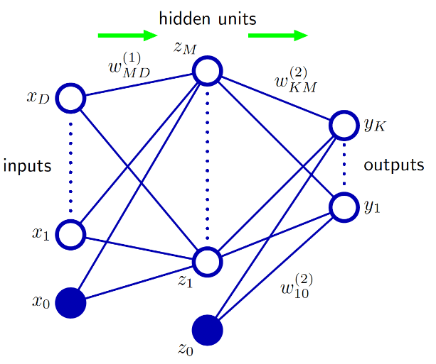
Figure5 Feed-forward neural network [6]
Supervised Learning is concerned with predicting an output for a given input. It is based on learning the relationship between inputs and outputs, using training data consisting in example input/output pairs, being divided into regression or classification, depending on the type of the output variable to be predicted (discrete or continuous). Support Vector Machine (SVM) or Regression (SVR), Artificial Neural Network (ANN, with the feed-forward step shown in Fig. 5), and Convolutional Neural Network (CNN) are examples of supervised learning.
Unsupervised learning is the task of finding patterns within data without the presence of any ground truth or labelling of the data, with a common unsupervised learning task being clustering (group of data points that are close to one another, relative to data points outside the cluster). Examples of unsupervised learning are the K-means and K-Nearest Neighbour (KNN) algorithms [7].
So far, ML algorithms have been applied to four key problems in weather prediction:
Correction of systematic error in NWP outputs, which involves post-processing data to remove biases [8]
Assessment of the predictability of NWP outputs, evaluating the uncertainty and confidence scores of ensemble forecasting [9]
Extreme detection, involving prediction of severe weather such as hail, gust or cyclones [10]
NWP parametrizations, replacing empirical models for radiative transfer or boundary-layer turbulence with ML techniques [11]
The first key problem, which concerns the correction of systematic error in NWPs, is the most popular area of application of ML methods in meteorology. In this field, wind speed and precipitation observational data are often used to perform an ML linear regression on the NWP data with the end goal of enhancing its accuracy and resolving local details of the weather which were unresolved by NWP forecasts. Although attractive for its simplicity and robustness, linear regression presents two problems: (1) least-square methods used to solve linear regression do not scale well with the size of datasets (since matrix inversion required by least square is increasingly expensive for increasing datasets size), (2) Many relationships between variables of interest are nonlinear. Instead, classification tree-based methods have proven very useful to model non-linear weather events, from thunderstorm and turbulence detection to extreme precipitation events, and the representation of the circular nature of the wind. In fact, compared to linear regression, random trees exhibit an easy scalability with large-size datasets which have several input variables. Besides preserving the scalability to large datasets of tree-based method, ML methods such as ANN and SVM/R provide also a more generic and more powerful alternative for nonlinear-processes modelling. These improvements have come at the cost of a difficult interpretation of the underlying physical concepts that the model can identify, which is critical given that scientists need to couple these ML models with physical-equations based NWP for variable interdependence. As a matter of fact, it has proven challenging to interpret the physical meaning of the weights and nonlinear activation functions that describe in the ANN model the data patterns and relationships found by the model [12].
The second key problem, represented by the interpretation of ensemble forecasts, is being addressed by ML unsupervised learning methods such as clustering, which represents the likelihood of a forecast aggregating ensemble members by similarity. Examples include grouping of daily weather phenomena into synoptic types, defining weather regimes from upper air flow patterns, and grouping members of forecast ensembles [13].
The third key problem, which concerns the prediction of weather extremes, corresponding to weather phenomena which are a hazard to lives and economic activities, ML based methods tend to underestimate these events. The problem here lies with imbalanced datasets, since extreme events represent only a very small fraction of the total events observed [14].
The fourth key problem to which ML is currently being applied, is parametrisation. Completely new stochastic ML approaches have been developed, and their effectiveness, along with their simplicity compared to traditional empirical models has highlighted promising future applications in (moist) convection [15]
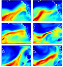
Further applications of ML methods are currently limited by intrinsic problems affecting the ML methods in relation to the challenges posed by weather data sets. While the reduction of the dimensionality of the data by ML techniques has proven highly beneficial for image pattern recognition in the context of weather data, it leads to a marked simplification of the input weather data, since it constrains the input space to individual grid cells in space or time [16]. The recent expansion of ANN into deep learning has provided new methodologies that can address these issues. This has pushed further the capability of ML models within the weather forecast domain, with CNNs providing a methodology for extracting complex patterns from large, structured datasets have been proposed, an example being the CNN model developed by Yunjie Liu in 2016 [17] to classify atmospheric rivers from climate datasets (atmospheric rivers are an important physical process for prediction of extreme rainfall events).
Figure 7 Sample images of atmospheric rivers correctly classified (true positive) by the deep CNN model in [18]
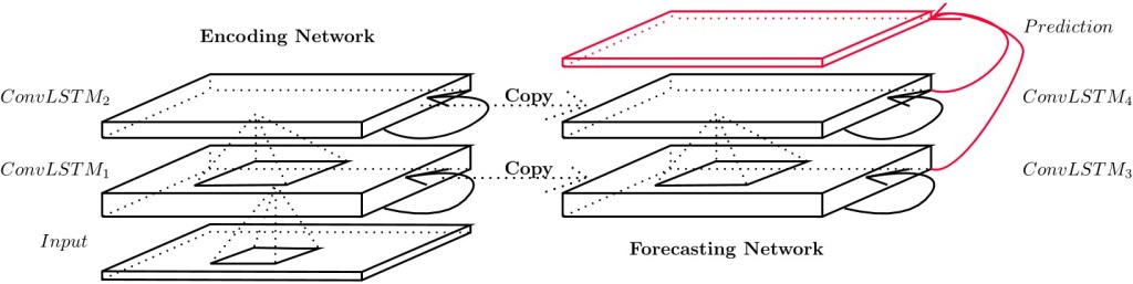
At the same time, Recursive Neural Networks (RNN), developed for natural language processing, are improving nowcasting techniques exploiting their excellent ability to work with the temporal dimension of data frames. CNN and RNN have now been combined, as illustrated in Fig. 6, providing the first nowcasting method in the context of precipitation, using radar data frames as input [18].
Figure 6 Encoding-forecasting ConvLSTM network for precipitation nowcasting [18]
While these results show a promising application of ML models to a variety of weather prediction tasks which extend beyond the area of competence of traditional NWPs, such as analysis of ensemble clustering, bias correction, analysis of climate data sets and nowcasting, they also show that ML models are not ready to replace NWP to forecast synoptic-scale and mesoscale weather patterns.
As a matter of fact, NWPs have been developed and improved for over 60 years with the very purpose to simulate very accurately and reliably the wind, pressure, temperature and other relevant prognostic fields, so it would be unreasonable to expect ML models to outperform NWPs on such tasks.
It is also true that, as noted earlier, the amount of available data will only grow in the coming decades, so it will be critical as well as strategic to develop ML models capable to extract patterns and interpret the relationships within such data sets, complementing NWP capabilities. But how long before an ML model will be capable to replace an NWP by crunching the entire set of historical observations of the atmosphere, extracting the patterns and the spatial-temporal relationships between the variables, and then performing weather forecasts?
Acknowledgement: I would like to thank my colleagues and friends Brian Lo, James Fallon, and Gabriel M. P. Perez, for reading and providing feedback on this article.
Buizza, R., Houtekamer, P., Pellerin, G., Toth, Z., Zhu, Y. and Wei, M. (2005) A comparison of the ECMWF, MSC, and NCEP global ensemble prediction systems. Mon Weather Rev, 133, 1076 – 1097
Lean, H. and Clark, P. (2003) The effects of changing resolution on mesocale modelling of line convection and slantwise circulations in FASTEX IOP16. Q J R Meteorol Soc, 129, 2255–2278
J. L. Aznarte and N. Siebert, “Dynamic Line Rating Using Numerical Weather Predictions and Machine Learning: A Case Study,” in IEEE Transactions on Power Delivery, vol. 32, no. 1, pp. 335-343, Feb. 2017, doi: 10.1109/TPWRD.2016.2543818.
Foley, Aoife M et al. (2012). “Current methods and advances in forecasting of wind power generation”. In: Renewable Energy 37.1, pp. 1–8.
McGovern, Amy et al. (2017). “Using artificial intelligence to improve real-time decision making for high-impact weather”. In: Bulletin of the American Meteorological Society 98.10, pp. 2073–2090
O’Gorman, Paul A and John G Dwyer (2018). “Using machine learning to parameterize moist convection: Potential for modeling of climate, climate change and extreme events”. In: arXiv preprint arXiv:1806.11037
Moghim, Sanaz and Rafael L Bras (2017). “Bias correction of climate modeled temperature and precipitation using artificial neural networks”. In: Journal of Hydrometeorology 18.7, pp. 1867–1884.
Camargo S J, Robertson A W Gaffney S J Smyth P and M Ghil (2007). “Cluster analysis of typhoon tracks. Part I: General properties”. In: Journal of Climate 20.14, pp. 3635–3653.
Ahijevych, David et al. (2009). “Application of spatial verification methods to idealized and NWP-gridded precipitation forecasts”. In: Weather and Forecasting 24.6, pp. 1485–1497.
Berner, Judith et al. (2017). “Stochastic parameterization: Toward a new view of weather and climate models”. In: Bulletin of the American Meteorological Society 98.3, pp. 565–588.
Fan, Wei and Albert Bifet (2013). “Mining big data: current status, and forecast to the future”. In: ACM sIGKDD Explorations Newsletter 14.2, pp. 1–5
Liu, Yunjie et al. (2016). “Application of deep convolutional neural networks for detecting extreme weather in climate datasets”. In: arXiv preprint arXiv:1605.01156.
Xingjian, SHI et al. (2015). “Convolutional LSTM network: A machine learning approach for precipitation nowcasting”. In: Advances in neural information processing systems, pp. 802–810.
In a recent blog post, I discussed the use of the analogue ensemble (AnEn), or “similar-day” approach to forecasting geomagnetic activity. In this post I will look at the use of support vector machines (SVMs), a machine learning approach, to the same problem and compare the performance of the SVM to the AnEn. An implementation of the SVM has been developed for this project in python and is available at https://doi.org/10.5281/zenodo.4604485.
Space weather encompasses a range of impacts on Earth caused by changes in the near-earth plasma due to variable activity at the Sun. These impacts include damage to satellites, interruptions to radio communications and damage to power grids. For this reason, it is useful to forecast the occurrence, intensity and duration of heightened geomagnetic activity, which we call geomagnetic storms.
As in the previous post, the measure of geomagnetic activity used is the aaHindex which has been developed by Mike Lockwood in Reading. The aaH index gives a global measure of geomagnetic activity at a 3-hour resolution. In this index, the minimum value is zero and larger values represent more intense geomagnetic activity.
The SVM is a commonly used classification algorithm which we implement here to classify whether a storm will occur. Given a sample of the input and the associated classification labels, the SVM will find a function that separates these input features by their class label. This is simple if the classes are linearly separable, as the function is a hyperplane. The samples lying closest to the hyperplane are called support vectors and the distance between these samples and the hyperplane is maximised.
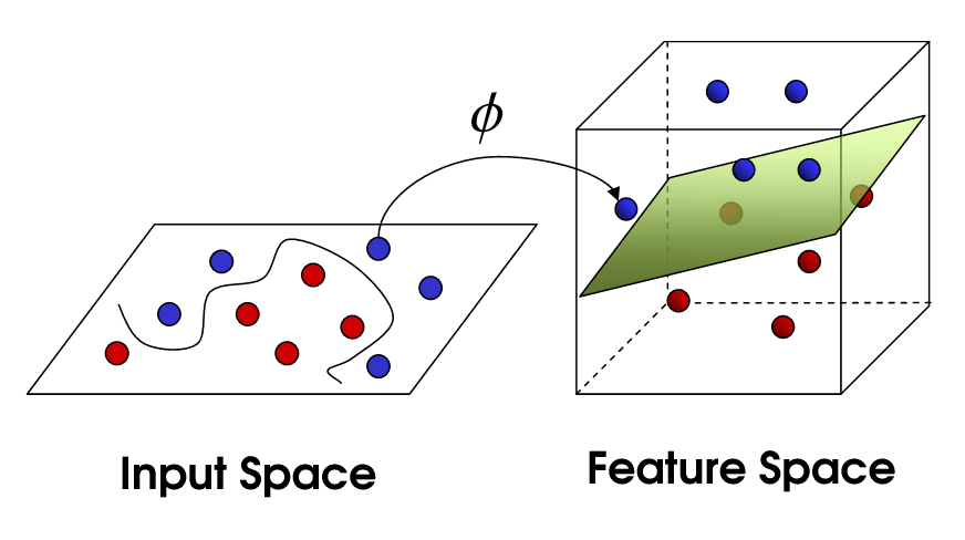
Figure 1 – A diagram explaining the kernel trick used by SVMs. This figure has been adopted from (Towards data science, n.d.)
Typically, the samples are not linearly separable, so we employ Cover’s theorem which states that linearly inseparable classification problems are more likely to be linearly separable when cast non-linearly into a higher dimensional space. Therefore, we use a kenel trick to throw the inputs into a higher dimensional feature space, as depicted in Figure 1, to make it more separable. Further explanation is available in (Towards data science, n.d.)
Based on aaH values in the 24-hour training window, the SVM predicts whether the next 3 hours will be either a storm or not. By comparing this dichotomous hindcast with the observed aaH, the outcome will be one of True Positive (TP, where a storm is correctly predicted), True Negative (TN, where no storm is correctly predicted), False Positive (FP, where a storm is predicted but not observed), or False Negative (FN, where a storm is not predicted but is observed). This is shown in the form of a contingency table in Figure 2.
Figure 2 – Contingency table for the SVM classifying geomagnetic activity into the “no-storm” and “storm” classes. THe results have been normalised across the true label.
For development of the SVM, the aaH data has been separated into independent training and test intervals. These intervals are chosen to be alternate years. This is longer than the auto-correlation in the data (choosing, e.g. alternate 3-hourly data points, would not generate independent training and test data sets) but short enough that we assume there will not be significant aliasing with solar cycle variations.
Training is an iterative process, whereby a cost function is minimised. The cost function is a combination of the relative proportion of TP, TN, FP and FN. Thus, while training itself, an SVM attempts to classify labelled data i.e., data belonging to a known category, in this case “storm” and “no storm” on the basis of the previous 24 hours of aaH. If the SVM makes an incorrect prediction it is penalised through a cost function which the SVM minimises. The cost parameter determines the degree to which the SVM is penalised for a misclassification in training which allows for noise in the data.
It is common that data with a class imbalance, that is containing many more samples from one class than the other, causes the classifier to be biased towards the majority class. In this case, there are far more non-storm intervals than storm intervals. Following (McGranaghan, Mannucci, Wilson, Mattman, & Chadwick, 2018), we define the cost of mis-classifying each class separately. This is done through the weight ratio Wstorm : Wno storm. Increasing the Wstorm increases the frequency at which the SVM predicts a storm and it follows that it predicts no storm at a reduced frequency. In this work we have varied Wstorm and kept Wno storm constant at 1. A user of the SVM method for forecasting may wish to tune the class weight ratio to give an appropriate ratio of false alarms and hit rate dependent on their needs.
Different forecast applications will have different tolerances for false alarms and missed events. To accommodate this, and as a further comparison of the hindcasts, we use a Cost/Loss analysis. In short, C is the economic cost associated with taking mitigating action when an event is predicted (whether or not it actually occurs) and L is the economic loss suffered due to damage if no mitigating action is taken when needed. For a deterministic method, such as the SVM, each time a storm is predicted will incur a cost C. Each time a storm is not predicted but a storm occurs a loss L is incurred. If no storm is predicted and no storm occurs, then no expense in incurred. By considering some time interval, the total expense can be computed by summing C and L. Further information, including the formular for computing the potential economic value (PEV) can be found in (Owens & Riley, 2017).
A particular forecast application will have a C/L ratio in the domain (0,1). This is because a C/L of 0 would mean it is most cost effective to take constant mitigating action and a C/L of 1 or more means that mitigating action is never cost effective. In either case, no forecast would be helpful. The power of a Cost/Loss analysis is that it allows us to evaluate our methods for the entire range of potential forecast end users without specific knowledge of the forecast application requirements. End users can then easily interpret whether our methods fit their situation.
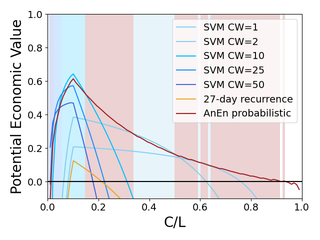
Figure 3 – A cost loss analysis comparing the potential economic value of a range of SVMs to the AnEn.
Figure 3 shows the potential economic value (PEV) of the SVM with a range of class weights (CW), probabilistic AnEn and 27-day recurrence. The shaded regions indicate which hindcast has the highest PEV for that Cost/Loss ratio. The probabilistic AnEn has the highest PEV for the majority of the Cost/Loss domain although SVM has higher PEV for lower Cost/Loss ratios. It highlights that the `best’ hindcast is dependent on the context in which it is to be employed.
In summary, we have implemented an SVM for the classification of geomagnetic storms and compared the performance to that of the AnEn which was discussed in a previous blog post. The SVM and AnEn generally perform similarly in a Cost/Loss analysis and the best method will depend on the requirements of the end user. The code for the SVM is available at https://doi.org/10.5281/zenodo.4604485 and the AnEn at https://doi.org/10.5281/zenodo.4604487.
References
Burges, C. (1998). A tutorial on support vector machines for pattern recognition. Data mining an knowledge discovery.
McGranaghan, R., Mannucci, A., Wilson, B., Mattman, C., & Chadwick, R. (2018). New Capabilities for Prediction of High-Latitude Ionospheric Scin-669tillation: A Novel Approach With Machine Learning. Space Weather.
Owens, M., & Riley, P. (2017). Probabilistic Solar Wind Forecasting Using Large Ensembles of Near-Sun Conditions With a Simple One-Dimensional “Upwind” Scheme. Space weather.