Prof. Tapio Schneider – Our Distinguished PhD Visiting Scientist.

Email: j.f.talib@pgr.reading.ac.uk

Every year PhD students from the Department of Meteorology at the University of Reading welcome a distinguished scientist in the field of environmental sciences. Previous scientists include Richard Rotunno (UCAR), Isaac Held (GFDL) and Susan Solomon (NOAA). This year’s honoured visitor was Professor Tapio Schneider from the climate dynamics research group from California Institute of Technology (Caltech), the academic home of NASA’s Jet Propulsion Laboratory. Tapio is a well-known contributor to our understanding of global climate dynamics and it was a pleasure to welcome him to our department.

SAMSUNG CSC
Prof. Tapio Schneider with some of the current PhD cohort.

Our visiting scientist programme in the department is an opportunity for PhD students to share and explain their research to an external visitor. It allows for PhD research to be looked at from a completely new perspective which will hopefully improve the PhD studies. In a typical PhD visiting scientist week, the visiting scientist meets students one to one, attends departmental research groups and presents work in departmental seminars.

Tapio Schneider presented two departmental seminars during his time with us titled How low clouds respond to warming: Observational, numerical and physical constraints and Model hierachies: From advancing climate dynamics to improving predictions. The latter of these seminars encouraged a discussion to rethink how we approach advancing our modelling capabilities. Tapio argued that the atmospheric modelling community had not fully engaged in the benefits that observations offer. He suggested that our goal should be a heirarchical system that integrates both observational data and models. We should look into creating “machine-learning” models, those which use observational data to improve our modelling capabilities through altering parameterisation schemes and radiative balance calculations at the top of the atmosphere (as two examples).

As already mentioned, the visiting scientist also meets with students one-to-one and it was highly beneficial for my own project to have a meeting with Tapio Schneider. We discussed papers released by himself alongside his former PhD student Tobias Bischoff (for example, The Equatorial Energy Balance, ITCZ position and Double-ITCZ bifurications) which concentrate on creating a diagnostic framework with which we can estimate the location and structure of the Inter-Tropical Convergence Zone (ITCZ). We discussed conclusions reached from my own aquaplanet simulations and how they relate to the proposed diagnostic framework. Keep an eye on the blog for a post coming soon on the developments in my own PhD project, (titled, what determines the location and intensity of the ITCZ?).

To bring this blog post to a close I would like to thank Professor Tapio Schneider for his time, knowledge and wisdom that he shared with the PhD cohort whilst at Reading. Thank you also to those from the University of Reading who supported Tapio’s visit. Feedback from the PhD cohort is extremely positive and I would highly recommend a similar scheme for other scientific departments.

20170508_193056
PhD social with the distinguished visitor.

Under-ice melt ponds in the Arctic

Email: n.e.smith@pgr.reading.ac.uk

The Arctic’s climate is one of those most rapidly changing globally, and as such the region has become a poster-child of climate change. Sea ice area is frequently used as an indicator of the rate of change of the system, providing striking visualisations of the rapidity of the change in recent years. The sea ice is also a driver of climate change, with areal cover greatly affecting the planet’s albedo and ice melt cooling and desalinating the Arctic ocean, altering circulation globally.

meltwaterLayerHHopNorskPolarinstitutt

Photo: Haakon Hop, Norsk Polarinstitutt

During the summer months, incoming solar radiation melts the surface layers of the sea ice. This melt water collects in hollows on the surface of the sea ice forming pools called melt ponds. Since the sea ice is porous, water from these ponds can percolate down or flow down through macroscopic flaws in the ice and out of the base of the ice. The melt water is relatively warm and fresh compared to the ocean below, so it floats between the ice and the ocean, gathering in pools beneath the sea ice called under-ice melt ponds. [1]

A couple of types of ice growth have been observed associated with these ponds. Most importantly, a sheet of ice can form at the interface between the pond and the ocean, completely isolating the fresh water from the ocean. As they create the illusion that they are the base of the sea ice, these sheets of ice are commonly referred to as ‘false bottoms’. [2]

We have developed a one-dimensional thermodynamic model of under-ice melt ponds to investigate how they affect their surroundings. We have carried out a number of sensitivity studies using this model, which have lead to some interesting conclusions about how these ponds evolve and affect the ice above them.

For example, the thicker the sea ice above an under-ice melt pond, the longer it takes to freeze due to a shallower temperature gradient above. As a result, more ice is gained due to under-ice melt ponds beneath thicker ice. This could be a positive feedback cycle, since we expect to see thinner ice on average as the Arctic warms, leading to less ice gained due to the ponds beneath it.

eguSens0

We also see that, as well as the outcome observed in the field, in which the false bottom migrates upwards and thickens as it freezes through the pond, it can also ablate under certain conditions. For example, ponds that are relatively salty at the start of the simulation freeze more slowly, and the false bottom ablates before it is able to reach the base of the sea ice.

eguSens1

Our sensitivity studies show that under-ice melt ponds could be responsible for up to 7.9% additional ice thickness at the end of a 50 day simulation. This would equate to up to 3.2% more ice volume across the Arctic dependent on the area of the ice underlain by these pools.

Recently, we have coupled our under-ice melt pond model with a simple, zero-dimensional model of the oceanic mixed layer. Using this coupled model, we see that the false bottom ablates more rapidly than a slab of sea ice, releasing more fresh water into the mixed layer. This strong reduction of salinity causes a shallowing of the mixed layer. We are currently further investigating the effects that the ponds have on the ocean below them.

Under-ice melt ponds and false bottom insulate the sea ice from below and affect the basal fluxes of salt and fresh water into the mixed layer, and thicken the ice above them allowing less radiation to penetrate through from the surface. They are clearly significant to the mass balance of the ice and the ocean below them, yet are not currently accounted for in the sea ice components of climate models. A parameterisation of their effects would be useful to include.

[1] Notz, Dirk, et al. “Impact of underwater‐ice evolution on Arctic summer sea ice.” Journal of Geophysical Research: Oceans 108.C7 (2003).

[2] Martin, Seelye, and Peter Kauffman. “The evolution of under-ice melt ponds, or double diffusion at the freezing point.” Journal of Fluid Mechanics 64.3 (1974): 507-528.

A PhD Student’s Guide to EGU 2017

Email: r.frew@pgr.reading.ac.uk

EGU2017logo

Science is a community effort, requiring collaboration and lots of different people providing different parts of the jigsaw to try to understand more and more of the full picture. Despite a lot of research being carried out individually in a lab, or at a desk, no one individual can do everything themselves, no matter how much of a genius they are. Sharing, discussing and debating are key to the progression of scientific ideas, and this ethos is something large scientific conferences like EGU cultivates.

Attending EGU for the first time as a PhD student was both an exciting and overwhelming experience due to its shear size and number of people. This year 14,496 people from 107 countries participated, giving 4,849 talks, 11,312 posters and 1,238 PICO presentations throughout the week!  

With 649 scientific sessions running throughout the week, deciding how to spend your day was a significant challenge in itself! The EGU website and app allowed you to create a personal programme, cutting down the number of entire printed programmes being printed, aiming to try to make EGU slightly more environmentally friendly.

IMG_2541
Vienna international conference centre, image courtesy of Matt Priestley.

A ‘typical’ day at EGU consisted of something like… 

7-8am: Wake up, shower and breakfast and then hop on the U-bahn to the conference centre. Pick up a EGU Today newsletter on the way into the centre, highlighting a few sessions happening that day that may be of general interest

8.30-10am: Division session of your choice consisting of six 15min talks. People also pick out specific talks in different sessions and hop between, especially if their work is more interdisciplinary and covers a few different sessions.

10-10.30am: Recharge with a much needed coffee break!

10.30am-12pm: Go to a debate on ‘Make Facts Great Again: how can scientists stand up for science?‘ There were a number of other topical debates throughout the week, including ‘Arctic environmental change: global opportunities and threats‘ and ‘Great Debate on Great Extinctions‘. This consisted of a short introduction from members of a panel, then questions from the floor.

12-1.30pm: Pick up something for lunch from one of the nearby bakeries or cafes around the conference centre, and sit in the nearby park and enjoy the sunshine (hopefully).

1.30-3pm: Explore the many information stands in the exhibition areas. These included publishing houses, geoscience companies, NGOs etc. Next go and vote in the EGU photograph competition: https://imaggeo.egu.eu/photo-contest/2017/, before stopping to listen to some PICO (Presenting Interactive COntent) presentations. These are very interactive sessions where speakers give a 2min overview of their work, after which people have the opportunity to go and question speakers further afterwards by a poster/couple of slides.

3-3.30pm: Tea/coffee break with cookies in the Early Career Scientists lounge.

3.30-5pm: Polar Science Career Session aimed at Early Career Scientists (there were also sessions for other divisions), consisting of an informal Q&A with a panel covering a variety of different career paths.

5-7pm: Poster sessions in the big halls with beer/juice and nibbles. These were a great opportunity for in depth discussion, and meeting other people in your field.

7-8.30pm: Early career scientist (ECS) reception with drinks and canapes, meet other ECS from all fields and chat with division leaders. This year 53% of EGU participants were ECSs, and there was a definite effort to cater for them throughout the week.

8.30-?: Dinner and drinks in Vienna town centre with peers, followed by an early night if you plan to make it to a 8.30am session tomorrow…

EGU2017photowinners
EGU 2017 photo competition entries, image taken from the GeoLog blog, more information about the entries and results can be found at: http://blogs.egu.eu/geolog/2017/04/28/at-the-assembly-2017-friday-highlights/

In addition to events highlighted, there were also a variety short courses running, for example ‘Tips and Tricks: How to Navigate EGU‘, ‘How to write a research grant‘ or ‘Rhyme your Research‘! EGU had its own official blog GeoLog, highlighting some of the events from each day: http://blogs.egu.eu/geolog/.

However, EGU is 5 days long, and despite the impressive offering of sessions being put on it would be a shame to go to Vienna and only see the conference centre… The odd extended lunch break to take the U-bahn (included as part of the entrance to the conference) to walk around the centre, or an afternoon off to explore a gallery or museum, or simply sit in one of the beautiful parks or cafes to enjoy some coffee and Sachertorte is definitely a must to recharge and finish off the week!

The onset and end of wet seasons over Africa

Email: c.m.dunning@pgr.reading.ac.uk

For many Africans, the timing of the wet season is of crucial importance, especially for those reliant upon subsistence agriculture, who depend on the seasonal rains for crop irrigation. In addition, the wet season recharges lakes, rivers and water storage tanks which constitute the domestic water supply in some areas. The timing of the wet season also affects the availability of energy from hydroelectric schemes, and has impacts upon the prevalence of certain disease carrying vectors, such as mosquitoes.

Climate change is already threatening many vulnerable populations, and changes in the timing or intensity of the wet season, or increasing uncertainty in the timing of the onset, may lead to significant socio-economic impacts. But before we consider future projections or past changes in the seasonality, we need to go back a few steps.

The first step is to find a method for determining when the wet season starts and ends (its ‘onset’ and ‘cessation’). In order to look at large-scale shifts in the timing of the wet season and relate this to wider-scale drivers, this method needs to be applicable across the entirety of continental Africa. Most previous methods for determining the onset focus on the national to regional scale, and are dependent on the exceedance of a certain threshold e.g. the first week with at least 20mm of rainfall, with one rainfall event of more than 10mm, and no dry spell of more than 10 days after the rain event for the next month. While such definitions work well at a national scale they are not applicable at a continental scale where rainfall amounts vary substantially. A threshold suitable for the dry countries at the fringes of the Sahara would not be suitable in the wetter East African highlands.

In addition to a vast range of rainfall amounts, the African continent also spans multiple climatic regimes. The seasonal cycle of precipitation over continental Africa is largely driven by the seasonal progression of the ITCZ and associated rain belts, which follows the maximum incoming solar radiation. In the boreal summer, when the thermal equator sits between the equator and the Tropic of Cancer, the ITCZ sits north of the equator and West Africa and the Sahel experience a wet season. During the boreal autumn the ITCZ moves south, and southern Africa experiences a wet season during the austral summer, followed by the northward return of the ITCZ during the boreal spring. As a consequence of this, central African regions and the Horn of Africa experience two wet seasons per year – one as the ITCZ travels north, and a second as the ITCZ travels south. A method for determining the onset and cessation at the continental scale thus needs to account for regions with multiple wet seasons per year.

In our paper (available here) we propose such a method, based on the method of Liebmann et al (2012). The method has three steps:

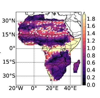
  • Firstly, determine the number of seasons experienced per year at the location (or grid point) of interest. This is achieved using harmonic analysis – the amplitude of the first and second harmonic were computed, using the entire timeseries and their ratio compared. If the ratio was greater than 1.0, i.e. the amplitude of the second harmonic was greater than the amplitude of the first harmonic then the grid point was defined as having two wet seasons per year (biannual), if the ratio was less than one then it was defined as having an annual regime. Figure 1 shows the ratio for one African rainfall dataset (TARCATv2). Three regions are identified as biannual regions; the Horn of Africa, an equatorial strip extending from Gabon to Uganda and a small region on the southern West African coastline.

    blog_fig1
    Figure 1: Location of regions with one and two seasons per year, determined using harmonic analysis. Yellow indicates two seasons per year, while pink/purple indicates one season per year. Computed from TARCATv2 data.
  • Secondly the period of the year when the wet season occurs was determined. This was achieved by looking for minima and maxima in the climatological cumulative daily rainfall anomaly to identify one or two seasons.
  • The third and final stage is to calculate the onset and cessation dates for each year. This is done by looking for the minima and maxima in the cumulative daily rainfall anomaly, calculated for each season.

Figure 2 shows the seasonal progression of the onset and cessation, with the patterns observed in agreement with those expected from the driving physical mechanisms, and continuous progression across the annual/biannual boundaries. Over West Africa and the Sahel, Figure 2a-b shows zonally-contiguous progression patterns with onset following the onset of the long rains and moving north, and cessation moving southward, preceding the end of the short rains. Over southern Africa Figure 2c-d shows the onset over southern Africa starting in the north-west and south-east, following the onset of the short rains, reaching the East African coast last, and cessation starting at the Zimbabwe, Mozambique, South Africa border and spreading out radially into the cessation of the long rains.

As well as testing the method for compatibility with known physical drivers of African rainfall, agreement across multiple satellite-based rainfall estimates was also examined. In general, good agreement was found across the datasets, particularly for regions with an annual regime and over the biannual region of East Africa.

blog_fig2
Figure 2: Southward and northward progression of the onset and cessation across the annual/biannual boundaries, computed using GPCP daily rainfall data 1998-2013.

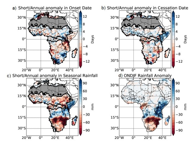
The advantage of having a method that works at the continental scale is the ability to look at the impact of large-scale oscillations on wider-scale variability. One application of this method was to investigate the impact of El Niño upon both the annual rains and short rains (Figure 3). In Figure 3 we see the well-documented dipole in rainfall anomaly, with higher rainfall totals over 0–15°S and the Horn of Africa in El Niño years and the opposite between 15°S and 30°S.  This anomaly is stronger when we use this method compared with using standard meteorological seasons. We can also see that while the lower rainfall to the south is colocated with later onset dates and a consequentially shorter season, the higher rainfall over the Horn of Africa is associated with later cessation of the short rains, with only small differences in onset date.

blog_fig3
Figure 3: a-c) Composite of onset, cessation and wet season rainfall in El Niño years for annual rains and short rains, minus the mean over 1982-2013, computed using CHIRPS data d) Oct-Feb rainfall anomaly in  years (CHIRPS).

In addition to using this method for research purposes, its application within an operational setting is also being explored. Hopefully, the method will be included within the Rainwatch platform, which will be able to provide users with a probabilistic estimate of whether or not the season has started, based on the rainfall experienced so far that year, and historical rainfall data.

For more details, please see the paper detailing this work:

Dunning, C.M., E Black, and R.P. Allan (2016) The onset and cessation of seasonal rainfall over Africa, Journal of Geophysical Research: Atmospheres, 121 11,405-11,424, doi: 10.1002/2016JD025428

References:

Liebmann, B., I. Bladé, G. N. Kiladis, L. M. Carvalho, G. B. Senay, D. Allured, S. Leroux, and C. Funk (2012), Seasonality of African precipitation from 1996 to 2009, J. Clim.25(12), 4304–4322.

Industrial Sponsored Doctorates

Email: a.halford@pgr.reading.ac.uk

When it comes to doctoral funding, the current method means project funds can come from a variety of sources, such as research councils, charities, industry partners or a mixture of these. In this blog post I will talk about my experience of being jointly funded by a research council and industrial partner.

To start with, I am not actually a PhD student like most people in the Meteorology department here at the University of Reading, but an EngD student. An EngD is a more industrial focused PhD, based on collaboration between industry and academia. There is a taught element to an EngD in the first year, during which a range of modules are covered, on everything from business analysis to sustainability. Additionally, a portion of time is dedicated to work for the industrial sponsor during the course of the project. An EngD still has the same end goal of a PhD, of an intellectual contribution to knowledge.

EngDs were started by the Engineering and Physical Sciences Research Council (EPSRC) back in 1992 and after initial success, the program was expanded in 2009. Out of this expansion came the Technologies for Sustainable Built Environments (TSBE) Centre at the University of Reading. The TSBE Centre has produced 40 EngDs over 8 years, covering a wide variety of disciplines, from modelling energy usage in the home to the effect of different roofing materials on bats. Each student is based within multiple academic departments and the industrial partner organisation with the aim of answering real world research questions.

My project is in collaboration with the BT Group and looks at weather impacts on the UK telecommunications network. I have found that being in an industrial sponsored project is of great benefit. It has been useful to get experience of how industry works, as it can be very different to the academic life in which most doctoral students find themselves. There have also been a lot of opportunities for training in specialist subjects including industrial project management and help to get chartership from professional bodies for those who want it. Being linked with an industrial partner can also offer strong networking and knowledge transfer opportunities, as was the case when I attended a recent interdisciplinary conference of the newly formed Tommy Flowers Institute. This institute has been formed by BT, along with other partner organisations, to further support collaboration between industry and academia.

It can be a challenge at times to balance the approaches of academia and industry. They do not always pull you in the same direction but this is often the same with any lengthy piece of work produced under the guidance of different advisors from different disciplines. The strength with the EngD partnership comes from the different perspectives offered from those different fields to ultimately solve the problem in question.

For me working on a heavily applied problem in the setting of a real organisation has been of greater benefit to me than working on a purely theoretical problem would have been. I have enjoyed seeing my preliminary output being tested within the organisation and look forward to being able to test a more advanced version in the final stages of my project.

Alan Halford is funded by the EPSRC and BT and supported by the TSBE centre.


Innovating for Sustainable Development

Email: Rachael.Byrom@pgr.reading.ac.uk

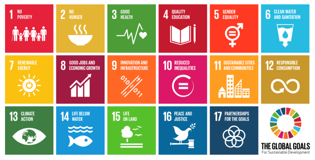
In 2016 the United Nations (UN) Sustainable Development Goals (SDGs) officially came into force to tackle key global challenges under a sustainable framework.

The SDGs comprise 17 global goals and 169 targets to be achieved across the next 15 years. As part of the ‘2030 Agenda’ for sustainable development, these goals aim to address a range of important global environmental, social and economic issues such as climate change, poverty, hunger and inequality. Adopted by leaders across the world, these goals are a ‘call for action’ to ensure that no one is left behind. However, the SDGs are not legally binding. The success of goals will rely solely on the efforts of individual countries to establish and implement a national framework for achieving sustainable development.

UN SDGs
The United Nation’s 17 Sustainable Development Goals

As part of the NERC funded ‘Innovating for Sustainable Development’ programme, students here in the Department of Meteorology were given the opportunity to explore and find solutions to key environmental challenges as outlined in the UN’s SDGs.

Run by the SCENARIO and SSCP doctoral training partnerships, the programme challenged students from a variety of disciplines and institutions to re-frame the SDGs from a multi-disciplinary perspective and to develop tangible, innovative solutions for sustainable development.

The programme began with an ‘Interdisciplinary Challenges Workshop’ where students participated in activities and exercises to review the importance of the SDGs and to consider their multi-disciplinary nature. Students were encouraged to think creatively and discuss issues related to each of the goals, such as: ‘Is this SDG achievable?’, ‘Are the goals contradictory?’ and ‘How could I apply my research to help achieve the SDGs?’

SDGs
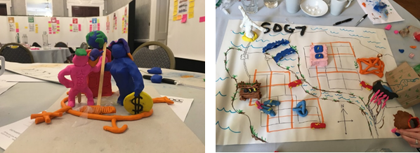
Visual representations of SDG 5 and SDG 7

Following this, three ‘Case Study’ days explored a handful of the SDGs in greater detail, with representatives from industry, start-ups and NGOs explaining how they are working to achieve a particular SDG, their current challenges and possible opportunities for further innovation.

The first Case Study day focused on both SDG 7 – Affordable and Clean Energy and SDG 12 – Responsible Consumption and Production. For SDG 7, insightful talks were given by the Moving Energy Initiative on the issue of delivering energy solutions to millions of displaced people, and BBOXX, on their work to produce and distribute off-grid solar power systems to rural communities in places such as Kenya and Rwanda. In the afternoon, presentations given by Climate-KIC start up NER and Waitrose showcased the efforts currently being taken to reduce wasteful food production and packaging, while Forum for the Future emphasised the importance of addressing sustainable nutrition.

The second Case Study day focused on SDG 6 – Clean Water and Sanitation. Experts from WaterAid, De-Solenator, Bear Valley Ventures, UKWIR and the International Institute for Environmental Development outlined the importance of confronting global sanitation and water challenges in both developing and developed nations. Alarmingly, it was highlighted that an estimated 40% of the global population are affected by water scarcity and 2.4 billion people still lack access to basic sanitation services, with more than 80% of human activity wastewater discharged into rivers without going through any stage of pollution removal (UN, 2016).

Case study
Participants discussing ideas during the second Case Study day

The last Case Study day explored SDG 9 – Industry, Innovation and Infrastructure and SDG 11 – Sustainable Cities and Communities. A range of talks on building technologies, carbon neutral buildings and sustainable solar technologies were given, along with a presentation by OPDC on the UK’s largest regeneration project. The day finished off with an overview from the Greater London Authority about the London Infrastructure Map and their new approach to sustainable planning and development across the city.

The programme finished off with a second workshop. Here students teamed up to develop innovative business ideas aimed at solving the SDG challenges presented throughout the Case Study events. Business coaches and experts were on hand to offer advice to help the teams develop ideas that could become commercially viable.

On the 16th March the teams presented their business ideas at the ‘Meet the Cleantech Pioneers’ networking event at Imperial’s new Translation and Innovation Hub (I-HUB). An overview of the projects can be found here. This event, partnered with the Climate-KIC accelerator programme, provided an excellent platform for participants to showcase and discuss their ideas with a mix of investors, entrepreneurs, NGOs and academics all interested in achieving sustainable development.

I-HUB
The final showcase event at Imperial’s I-HUB

Overall the programme provided a great opportunity to examine the importance of the SDGs and to work closely with PhD students from a range of backgrounds. Fundamentally the process emphasised the point that, in order for the world to meet the 2030 Agenda, many sustainable development challenges still need to be better understood and many solutions still need to be provided – and here scientific research can play a key role. Furthermore, it was made clear that a high level of interdisciplinary thinking, research and innovation is needed to achieve sustainable development.

Institutes

References:

UN, 2016: Clean Water and Sanitation – Why it matters, United Nations, Accessed 05 March 2017. [Available online at http://www.un.org/sustainabledevelopment/wp-content/uploads/2016/08/6_Why-it-Matters_Sanitation_2p.pdf]

Can we really use El Niño to predict flooding?

R. Emerton, H. Cloke, E. Stephens, E. Zsoter, S. Woolnough, F. Pappenberger (2017). Complex picture for likelihood of ENSO-driven flood hazard. Nature Communications. doi: 10.1038/NCOMMS14796

Email: r.e.emerton@pgr.reading.ac.uk

When an El Niño is declared, or even forecast, we think back to memorable past El Niños (such as 1997/98), and begin to ask whether we will see the same impacts. Will California receive a lot of rainfall? Will we see droughts in tropical Asia and Australia? Will Peru experience the same devastating floods as in 1997/98, and 1982/83?

news_headlines_elnino

El Niño and La Niña, which see changes in the ocean temperatures in the tropical Pacific, are well known to affect weather, and indeed river flow and flooding, around the globe. But how well can we estimate the potential impacts of El Niño and La Niña, and how likely flooding is to occur?

This question is what some of us in the Water@Reading research group at the University of Reading have been looking to answer in our recent publication in Nature Communications. As part of our multi- and inter-disciplinary research, we work closely with the Red Cross / Red Crescent Climate Centre (RCCC), who are working on an initiative called Forecast-based Financing (FbF, Coughlan de Perez et al.). FbF aims to distribute aid (for example providing water purification tablets to prevent spread of disease, or digging trenches to divert flood water) ahead of a flood, based on forecasts. This approach helps to reduce the impact of the flood in the first place, rather than working to undo the damage once the flood has already occurred.

Photo credit: Red Cross / Red Crescent Climate Centre

In Peru, previous strong El Niños in 1982/83 and 1997/98 had resulted in devastating floods in several regions. As such, when forecasts in early 2015 began to indicate a very strong El Niño was developing, the RCCC and forecasters at the Peruvian national hydrological and meteorology agency (SENAMHI) began to look into the likelihood of flooding, and what FbF actions might need to be taken.

Typically, statistical products indicating the historical probability (likelihood [%] based on what happened during past El Niños) of extreme precipitation are used as a proxy for whether a region will experience flooding during an El Niño (or La Niña), such as these maps produced by the IRI (International Research Institute for Climate and Society). You may also have seen maps which circle regions of the globe that will be drier / warmer / wetter / cooler – we’ll come back to these shortly.

These rainfall maps show that Peru, alongside several other regions of the world, is likely to see more rainfall than usual during an El Niño. But does this necessarily mean there will be floods? And what products are out there indicating the effect of El Niño on rivers across the globe?

For organisations working at the global scale, such as the RCCC and other humanitarian aid agencies, global overviews of potential impacts are key in taking decisions on where to focus resources during an El Niño or La Niña. While these maps are useful for looking at the likely changes in precipitation, it has been shown that the link between precipitation and flood magnitude is nonlinear (Stephens et al.),  – more rain does not necessarily equal floods – so how does this transfer to the potential for flooding?

The motivation behind this work was to provide similar information, but taking into account the hydrology as well as the meteorology. We wanted to answer the question “what is the probability of flooding during El Niño?” not only for Peru, but for the global river network.

To do this, we have taken the new ECMWF ERA-20CM ensemble model reconstruction of the atmosphere, and run this through a hydrological model to produce the first 20th century global hydrological reconstruction of river flow. Using this new dataset, we have for the first time estimated the historical probability of increased or decreased flood hazard (defined as abnormally high or low river flow) during an El Niño (or La Niña), for the global river network.

elnino_flood_hazard_gif_beccalize
Figure 1: The probability of increased (blue) or decreased (red) flood hazard during each month of an El Nino. Based on the ensemble mean of the ERA-20CM-R 20th century river flow reconstruction.

The question – “what is the probability of flooding during El Niño?”, however, remains difficult to answer. We now have maps of the probability of abnormally high or low river flow (see Figure 1), and we see clear differences between the hydrological analysis and precipitation. It is also evident that the probabilities themselves are often lower, and much more uncertain, than might be useful – how do you make a decision on whether to provide aid to an area worried about flooding, when the probability of that flooding is 50%?

blob_floodhazard_comparison_map
Figure 2: Historical probability of increased / decreased flood hazard map for February, with overlay showing the typical impact map for winter during an El Nino. This highlights the complexity of the link between El Nino and flooding compared to the information usually available.

The likely impacts are much more complex than is often perceived and reported – going back to the afore-mentioned maps that circle regions of the globe and what their impact will be (warmer, drier, wetter?) – these maps portray these impacts as a certainty, not a probability, with the same impacts occurring across huge areas. For example, in Figure 2, we take one of the maps from our results, which indicates the probability of increased or decreased flood hazard in one month during an El Niño, and draw over this these oft-seen circles of potential impacts. In doing this, we remove all information on how likely (or unlikely) the impacts are, smaller scale changes within these circles (in some cases our flood hazard map even indicates a different impact), and a lot of the potential impacts outside of these circles – not to mention the likely impacts can change dramatically from one month to the next. For those organisations that take actions based on such information, it is important to be aware of the uncertainties surrounding the likely impacts of El Niño and La Niña.

“We conclude that while it may seem possible to use historical probabilities to evaluate regions across the globe that are more likely to be at risk of flooding during an El Niño / La Niña, and indeed circle large areas of the globe under one banner of wetter or drier, the reality is much more complex.”

PS. During the winter of 2015/16, our results estimated an ~80% likelihood of increased flood hazard in northern coastal Peru, with only ~10% uncertainty surrounding this. The RCCC took FbF actions to protect thousands of families from potentially devastating floods driven by one of the strongest El Niños on records. While flooding did occur, this was not as severe as expected based on the strength of the El Niño. More recently, during the past few months (January – March 2017), anomalously high sea surface temperatures (SSTs) in the far eastern Pacific (known as a “coastal El Niño” in Peru but not widely acknowledged as an El Niño because central Pacific SSTs are not anomalously warm) have led to devastating flooding in several regions and significant loss of life. And Peru wasn’t the only place that didn’t see the impacts it expected in 2015/16; other regions of the world, such as the US, also saw more rainfall than normal in places that were expected to be drier, and California didn’t receive the deluge they were perhaps hoping for. It’s important to remember that no two El Niños are the same, and El Niño will not be the only influence on the weather around the globe. While El Niño and La Niña can provide some added predictability to the atmosphere, the impacts are far from certain.

Presidente Kuczynski recorre zonas afectadas por lluvias e inund
Flooded areas of Trujillo, Peru, March 2017. Photo credit: Presidencia Peru, via Floodlist

Full reference:

R. Emerton, H. Cloke, E. Stephens, E. Zsoter, S. Woolnough, F. Pappenberger (2017). Complex picture for likelihood of ENSO-driven flood hazard. Nature Communications. doi: 10.1038/NCOMMS14796

Press Release:

The Influence of the Weather on Bird Migration

Email: d.l.a.flack@pgr.reading.ac.uk

As well as being a meteorologist, I am a bird watcher. This means I often combine meteorology and bird watching to see the impact of the weather on birds. Now that we are well into March my focus in bird watching turns to one thing – the migration.

March generally marks the time when the first summer migrants start arriving into the UK. Already this year we have had reports of Sand Martin, Wheatear, Garganey, Little Ringed Plover, White Wagtail, Osprey, Swallow, House Martin, Ring Ouzel and Whitethroat (up to 9 March), some of which are depicted below.

Wheatear_PhDblog
Wheatear
Garganey_PhDgroup
Garganey
White_wagtail_PhDgroup
White Wagtail
OLYMPUS DIGITAL CAMERA
Swallow

There are many people that consider the arrival dates of certain migratory species of birds and how this arrival date changes over many years. I do keep extensive records of the birds that I see (and thus arrival dates), but what interests me more are the odd days in the record, and the sightings of unusual birds and working out how they arrived at their destinations.

A good example of this can be found by looking at my first Swallow sighting of the year in Kent and East Sussex. Since I started bird watching in 2001 my first Swallow of the year has moved from around 10 April to between 26-March and 1 April. However in 2013 my first record was 15 April. Then in 2015 and 2016 I saw my first Swallow on 1 April and 27 March respectively (I was in Cheshire in 2014 in late March/early April).

So what happened; why were the Swallows late in Kent in 2013? Well, it all comes down to wind direction. The spring of 2013 was very chilly and along the east coast there were plenty of N/NE winds – this would have provided a head wind so the Swallows would preferentially not migrate up the east coast in those conditions but instead migrate up the west coast where there were southerlies.

So, the wind direction plays a key part in the migration of birds. If conditions are for a tailwind or very light winds the birds will migrate; otherwise they will stay put. However, headwinds can lead to some interesting phenomena associated with bird migration – ‘falls’.

A ‘fall’ occurs when there are a large number of migrants building up along the coastline at a departure point (so for the interest of UK bird watchers Northern France), as they cannot get to their destination. When the wind direction changes the birds will then migrate en masse and quite literally fall out of the sky.

It’s not all about the wind direction though; rain is also a key factor that bird watchers consider when looking at weather forecasts. Essentially, fronts and showers are great for bird watchers. On migration birds will often fly higher than they normally would. This means on a clear sunny day you could easily miss birds passing overhead as they are so high up. However, with the rain the birds will often fly lower, avoiding the in-cloud turbulence. For many of the summer migrants their food sources (insects) also fly lower in these conditions.

This means that a forecast of showers with a southerly wind is generally what I look for from mid-April onwards (particularly as an inland birder), as it means there is a good chance of migratory species turning up – also because then I can head out after work as the evenings are brighter. This is something that I did last year and ended up recording the first Sandwich Tern (photo below (not of the bird I saw)) of the year in Berkshire.

sandwich_tern_PhDblog
Sandwich Tern

So in summary, it’s not as simple as just keeping an eye on the wind direction – there are other factors that can influence the birds’ migration and where they will end up. For more information about the impact of weather on bird sightings (considering both rare and common birds) check out my blog.