Exploring the impact of variable floe size on the Arctic sea ice

Email: a.w.bateson@pgr.reading.ac.uk

The Arctic sea ice cover is made up of discrete units of sea ice area called floes. The size of these floes has an impact on several sea ice processes including the volume of melt produced at floe edges, the momentum exchange between the sea ice, ocean, and atmosphere, and the mechanical response of the sea ice to stress. Models of the sea ice have traditionally assumed that floes adopt a uniform size, if floe size is explicitly represented at all in the model. Observations of floes show that floe size can span a huge range, from scales of metres to tens of kilometres. Generally, observations of the floe size distribution (FSD) are fitted to a power law or a combination of power laws (Stern et al., 2018a).

The Los Alamos sea ice model, hereafter referred to as CICE, usually assumes a fixed floe size of 300 m. We can impose a simple FSD model into CICE derived from a power law to explore the impact of variable floe size on the sea ice cover. Figure 1 is a diagram of the WIPoFSD model (Waves-in-Ice module and Power law Floe Size Distribution model), which assumes a power law with a fixed exponent,
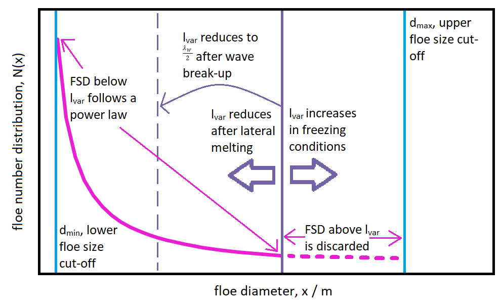
 \alpha, between a lower floe size cut-off, d_{min}, and an upper floe size cut-off, d_{max}. The model also incorporates a floe size variable, l_{var}, to capture the effects of processes that can influence floe size. The processes represented are wave break-up of floes, melting at the floe edge, winter floe growth, and advection. The model includes a wave advection and attenuation scheme so that wave properties can be determined within the sea ice field to enable the identification of wave break-up events. Full details of the WIPoFSD model and its implementation into CICE are available in Bateson et al. (2020). For the WIPoFSD model setup considered here, we explore the impact of the FSD on the lateral melt rate, which is the melt rate at the edge surfaces of floes. It is useful to define a new FSD metric that can be used to characterise the impact of the FSD on lateral melt. To do this we note that the lateral melt volume produced by a floe is proportional to the perimeter of the floe. The effective floe size, l_{eff}, is defined as a fixed floe size that would produce the same lateral melt rate as a given FSD, for a fixed total sea ice area.

Figure 1: A schematic of the imposed FSD model. This model is initiated by prescribing a power law with an exponent, \alpha, and between the limits d_{min} and d_{max}. Within individual grid cells the variable FSD tracer, l_{var}, varies between these two limits. l_{var} evolves through lateral melting, wave break-up events, freezing, and advection.

Here we will compare a CICE simulation incorporating the WIPoFSD model, hereafter referred to as stan-fsd, to a reference case, ref, using the CICE standard fixed floe size of 300 m. For the WIPoFSD model, d_{min} = 10 m, d_{max} = 30 km, and \alpha = -2.5. These values have been selected as representative values from observations. The reference setup is initiated in 1990 and spun-up until 2005, when either continued as ref or the WIPoFSD model imposed for stan-fsd before being evaluated from 2006 – 2016. All figures in this post are given as a mean over 2007 – 2016, such that 2005 – 2006 is a period of spin-up for the incorporated WIPoFSD model.

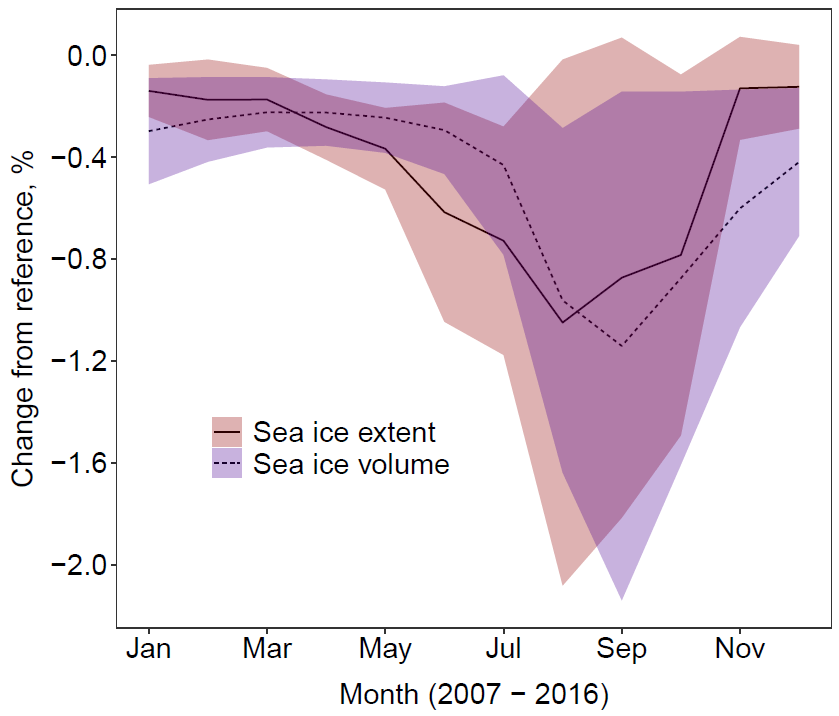
In Figure 2, we show the percentage reduction in the Arctic sea ice extent and volume of stan-fsd relative to ref. The differences in both extent and volume over the pan-Arctic scale evolve over an annual cycle, with maximum differences of -1.0 % in August and -1.1 % in September respectively. The annual cycle corresponds to periods of melting and freeze-up and is a product of the nature of the imposed FSD. Lateral melt rates are a function of floe size, but freeze-up rates are not, hence model differences only increase during periods of melting and not during periods of freeze-up. The difference in sea ice extent reduces rapidly during freeze-up because this freeze-up is predominantly driven by ocean surface properties, which are strongly coupled to atmospheric conditions in areas of low sea ice extent. In comparison, whilst atmospheric conditions initiate the vertical sea ice growth, this atmosphere-ocean coupling is rapidly lost due to insulation of the warmer ocean from the cooler atmosphere once sea ice extends across the horizontal plane. Hence a residual difference in sea ice thickness and therefore volume propagates throughout the winter season. The interannual variability shows that the impact of the WIPoFSD model with standard parameters varies significantly depending on the year.

Figure 2: Difference in sea ice extent (solid, red ribbon) and volume (dashed, blue ribbon) between stan-fsd relative to ref averaged over 2007–2016. The ribbon shows the region spanned by the mean value plus or minus 2 times the standard deviation for each simulation. This gives a measure of the interannual variability over the 10-year period.

Although the pan-Arctic differences in extent and volume shown in Figure 2 are marginal, differences are larger when considering smaller spatial scales. Figure 3 shows the spatial distribution in the changes in sea ice concentration and thickness in March, June, and September for stan-fsd relative to ref in addition to the spatial distribution in l_{eff} for stan-fsd for the same months. Reductions in the sea ice concentration and thickness of up to 0.1 and 50 cm observed respectively in the September marginal ice zone (MIZ). Within the pack ice, increases in the sea ice concentration of up to 0.05 and ice thickness of up to 10 cm can be seen. To understand the non-uniform spatial impacts of the FSD, it is useful to look at the behaviour of l_{eff}. Regions with an l_{eff} greater than 300 m will experience less lateral melt than the equivalent location in ref (all other things being equal) whereas locations with an l_{eff} below 300 m will experience more lateral melt. In Figure 3 we see the transition to values of l_{eff} smaller than 300 m in the MIZ, hence most of the sea ice cover experiences less lateral melting for stan-fsd compared to ref.

Figure 3: Difference in the sea ice concentration (top row, a-c) and thickness (middle row, d-f) between stan-fsd and ref and l_{eff} 
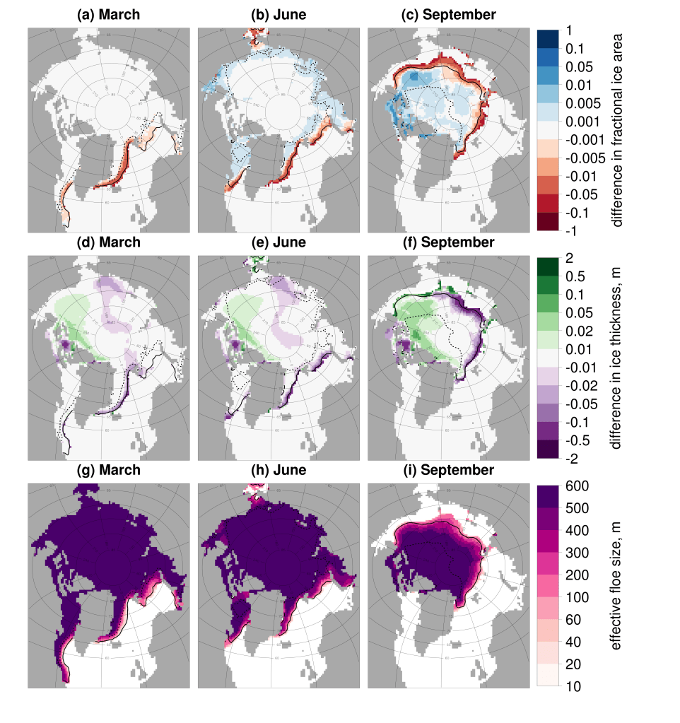
(bottom row, g-i) for stan-fsd averaged over 2007 – 2016. Results are presented for March (left column, a, d, g), June (middle column, b, e, h) and September (right column, c, f, i). Values are shown only in locations where the sea ice concentration exceeds 5 %.

For Figures 2-3, the parameters used to define the FSD have been set to fixed, standard values. However, these parameters vary significantly between different observed FSDs. It is therefore useful to explore the model sensitivity to these parameters. For α values of -2, -2.5, -3 and -3.5 have been selected to span the general range of values reported in observations (Stern et al., 2018a). For d_{min} values of 1 m, 20 m and 50 m are selected to reflect the different behaviours reported in studies, with some showing power law behaviour extending to 1 m (Toyota et al., 2006) and others showing a tailing off at an order of 10 s of metres (Stern et al., 2018b). For the upper cut-off, d_{max}, values of 1000 m, 10,000 m, 30,000 m and 50,000 m are selected, again to represent the distributions reported in different studies. 50 km is taken as the largest value for d_{max} as this serves as an upper limit to what can be resolved within an individual grid cell on a CICE 1^{\circ} grid. A total of 19 sensitivity studies have been completed used different permutations of the stated values for the FSD model parameters. Figure 4 shows the change in mean September sea ice extent and volume relative to ref plotted against mean annual l_{eff}, averaged over the sea ice extent, for each of these sensitivity studies. The impacts range from a small increase in extent and volume to large reductions of -22 % and -55 % respectively, even within the parameter space defined by observations. Furthermore, there is almost a one-to-one mapping between mean l_{eff} and extent and volume reduction. This suggests l_{eff} is a useful diagnostic tool to predict the impact of a given set of floe size parameters. The system varies most in response to the changes in the α, but it is also particularly sensitive to d_{min}.

Figure 4: Relative change (%) in mean September sea ice volume from 2007 – 2016 respectively, plotted against mean l_{eff} 
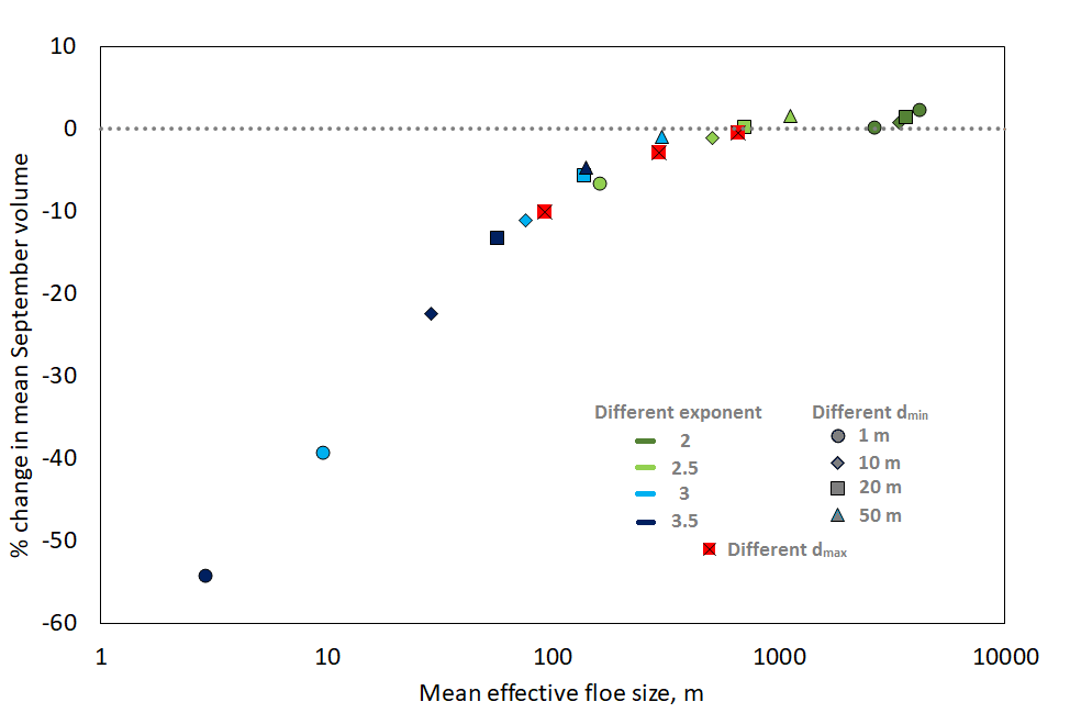
for simulations with different selections of parameters relative to ref. The mean l_{eff} is taken as the equally weighted average across all grid cells where the sea ice concentration exceeds 15%. The colour of the marker indicates the value of the \alpha, the shape indicates the value of d_{min}, and the three experiments using standard parameters but different d_{max} (1000 m, 10000 m and 50000 m) are indicated by a crossed red square. The parameters are selected to be representative of a parameter space for the WIPoFSD model that has been constrained by observations.

There are several advantages to the assumption of a fixed power law in modelling the sea ice floe size distribution. It provides a simple framework to explore the potential impact of an observed FSD on the sea ice mass balance, given observations of the FSD are generally fitted to a power law. In addition, the use of a simple model makes it easier to constrain the mechanism of how the model changes the sea ice cover. However, there are also significant disadvantages including the high model sensitivity to poorly constrained parameters, as shown in Figure 4. In addition, there is evidence both that the exponent evolves over an annual cycle and is not a fixed value (Stern et al., 2018b) and that the power law is not a statistically valid description of the FSD over all floe sizes (Horvat et al., 2019). An alternative approach to modelling the FSD is the prognostic model of Roach et al. (2018, 2019). The prognostic model avoids any assumptions about the shape of the distribution and instead assigns sea ice area to a set of adjacent floe size categories, with individual processes parameterised at floe scale. This approach carries its own set of challenges. If important physical processes are missing from the model it will not be possible to simulate a physically realistic distribution. In addition, the prognostic model has a significant computational cost. In practice, the choice of FSD modelling approach will depend on the application.

Further reading
Bateson, A. W., Feltham, D. L., Schröder, D., Hosekova, L., Ridley, J. K. and Aksenov, Y.: Impact of sea ice floe size distribution on seasonal fragmentation and melt of Arctic sea ice, Cryosphere, 14, 403–428, https://doi.org/10.5194/tc-14-403-2020, 2020.

Horvat, C., Roach, L. A., Tilling, R., Bitz, C. M., Fox-Kemper, B., Guider, C., Hill, K., Ridout, A., and Shepherd, A.: Estimating the sea ice floe size distribution using satellite altimetry: theory, climatology, and model comparison, The Cryosphere, 13, 2869–2885, https://doi.org/10.5194/tc-13-2869-2019, 2019. 

Stern, H. L., Schweiger, A. J., Zhang, J., and Steele, M.: On reconciling disparate studies of the sea-ice floe size distribution, Elem. Sci. Anth., 6, p. 49, https://doi.org/10.1525/elementa.304, 2018a. 

Stern, H. L., Schweiger, A. J., Stark, M., Zhang, J., Steele, M., and Hwang, B.: Seasonal evolution of the sea-ice floe size distribution in the Beaufort and Chukchi seas, Elem. Sci. Anth., 6, p. 48, https://doi.org/10.1525/elementa.305, 2018b. 

Roach, L. A., Horvat, C., Dean, S. M., and Bitz, C. M.: An Emergent Sea Ice Floe Size Distribution in a Global Coupled Ocean-Sea Ice Model, J. Geophys. Res.-Oceans, 123, 4322–4337, https://doi.org/10.1029/2017JC013692, 2018. 

Roach, L. A., Bitz, C. M., Horvat, C. and Dean, S. M.: Advances in Modeling Interactions Between Sea Ice and Ocean Surface Waves, J. Adv. Model. Earth Syst., 11, 4167–4181, https://doi.org/10.1029/2019MS001836, 2019.

Toyota, T., Takatsuji, S., and Nakayama, M.: Characteristics of sea ice floe size distribution in the seasonal ice zone, Geophys. Res. Lett., 33, 2–5, https://doi.org/10.1029/2005GL024556, 2006. 

A Journey through Hot British Summers

Email: s.h.lee@pgr.reading.ac.uk

The phrase “British summer” tends to evoke images of disorganised family barbecues being interrupted by heavy rain, or the covers coming on at Wimbledon, or the saying “three fine days and a thunderstorm”. Yet in recent years, hot weather has become an increasingly regular occurrence. Let me take you on a brief tour of notably hot summers in the UK. I’ll largely draw on the Met Office HadUK-Grid dataset, shown in Figure 1.

Figure 1: Nationally-averaged daily maximum temperatures for June-July-August from HadUK-Grid. In red is a 30-year centred running mean, which has risen by 1°C since the mid-20th century.

HadUK-Grid begins in 1884, but thanks to the Central England Temperature dataset (which extends back to 1659), we do have records of earlier heatwaves.  These include the hot summer of 1666, which set the scene for the Great Fire of London in September. The summers of 1781, 1826 and 1868 were also particularly hot. The first hot summer in the HadUK-Grid series is 1899, which was the warmest summer by average maxima in that series until 1976!

But our journey properly begins in 1911, when the temperature reached 36.7°C on August 9th. At the time, this was the highest reliably recorded temperature measured in the UK. It is hard to imagine how this summer must have felt at the time – not least in the cooler average climate, but also with the less developed infrastructure and clothing customs of the time. As with any heatwave, its impacts were large with increased death, drought, and agricultural impacts. The summer of 1911 was followed by the summer of 1912, which was the 2nd wettest on record for the UK. Such a turnaround must have been equally hard to believe and does highlight that extreme swings in the British weather are not, in themselves, new. In a series from 1884, the summer of 1911 is the 8th warmest in terms of the UK average maximum temperature (at the time, it would have been 2nd, with only 1899 warmer).

Stopping briefly in 1933 (which eclipsed 1911, but pales in comparison with the dustbowl conditions being experienced in the US at the time) and then again in August 1947 (which remains 2nd warmest for UK average maxima and the nation’s driest, and was in huge contrast to the tremendously snowy and cold February), our next destination is 1975.

1975 currently ranks as the 11th warmest for UK average maxima but is also the 19th driest. This, when combined with the dry winter that followed, set the scene for the infamous summer of 1976. Both these summers followed a spell of very cool summers, with no particularly remarkable summers in the 1960s, while the UK did not see a temperature above 28°C in 1974 (almost unthinkable nowadays). I won’t go into huge detail about the 1976 summer, but it is engrained in the minds of a generation thanks not only to its remarkable June heatwave (which has never been matched) but also the cool climate in which it occurred. It ranks as the 2nd driest summer for the UK and remains the warmest on record in terms of average maxima – though no individual month holds the number 1 spot.

Let us next whizz off to July 1983, which at the time had the warmest nationally averaged maxima for the month (it now ranks 3rd). Oddly enough, while the UK baked in heat, the temperature at Vostok, Antarctica dropped to -89.2°C on the 21st – the lowest surface-based temperature ever recorded. I am keeping the topic of this blog to hot summers, but I want to give 1985 a special mention – the most recent summer when the UK-average maxima were less than 17°C, a formerly frequent occurrence.

As we hot-foot it toward the end of the 20th century (pun intended), we arrive at 1990. Liverpool had just won the First Division (sound familiar?) and on August 3rd the temperature at Cheltenham, Gloucestershire reached 37.1°C – beating the record set in 1911 after 79 years. That night, the temperature fell to only 23.9°C in Brighton – the warmest night on record. However, the heatwave was rather brief but intense (3 consecutive days exceeded 35°C, the only other occurrences were in 1976). For a prolonged heatwave, we jump to August 1995. With a UK average maximum of 22.8°C, it remains the UK’s warmest August by that metric, and the 2nd driest. The summer ranks 2nd warmest by maxima. Soon after, the August of 1997 (4th warmest) added to growing evidence of a change to the British climate.

But it was in the August of 2003 when things really kicked off. In the earliest heatwave I remember, the temperature hit 38.5°C on the 10th at Faversham, Kent (satellite image in Figure 2) – the first time the UK had surpassed 37.8°C (100°F) and breaking the record from 1990 after only 23 years. 30°C was exceeded somewhere for 10 consecutive days. The summer of 2003 ranks nowadays as 6th warmest by average maxima; across Europe conditions were more extreme with a huge estimated death toll.

Figure 2: Terra-MODIS imagery from 10 August 2003, when the UK first surpassed 100°F and most of Europe was experiencing an intense heatwave (via https://worldview.earthdata.nasa.gov/)

Only 3 years later, July 2006 set the record for the hottest month for the UK-average maxima (23.3°C), and set – at the time – a record for the highest-recorded July temperature (36.5°C at Wisley on the 19th). Ranking 4th warmest by average maxima, the summer was even more extreme across mainland Europe.

What followed from 2007 through 2012 was a spell of wet summers, but we shrug off all that Glastonbury mud to arrive at July 2013, which currently ranks as 4th warmest by average maxima and saw the longest spell of >28°C weather since 1997.

Skipping through in increasingly short steps, we arrive for a brief blast on July 1st, 2015 – when the July record from 2006 fell, with 36.7°C at Heathrow in an otherwise cool month. We hop over now to 2018…

The summer of 2018, memorable for England’s performance in the World Cup, saw very warm temperatures in June and July. By nationally averaged maxima, June 2018 ranks 2nd behind 1940, and July sits 2nd behind 2006. The summer ranks 3rd, but by mean temperature is the warmest. Though not reaching the dizzying highs of 2003 (“only” 35.3°C was reached on July 26th), the prolonged dry conditions which began in May across England led to parched grasses (Figure 3), wildfires, and low river levels. I may have also had a viral tweet.

Figure 3: Brown grass during summer 2018 at the University of Reading, as seen in Google Earth.

With the present day in sight, our journey is not yet over. Stepping into 2019, an otherwise unremarkable summer was characterised with huge bursts of heat – setting records across Europe – which on July 25th saw the temperature reach 38.7°C at Cambridge Botanic Gardens. This eclipsed the 2003 record and became only the 2nd day – at the time – when 100°F or more had been reached in the UK.

But that is still not the end of the story! After a record-setting sunny spring followed by a mixed first half of summer, on July 31st 2020 the temperature at Heathrow hit 37.8°C – becoming the UK’s third warmest day on record and the third time 100°F had been recorded. The following Friday, 36.4°C was reached at Heathrow and Kew – the UK’s 9th warmest day on record, and highest temperature in August since 2003. Figure 4 shows the view at the University atmospheric observatory shortly after 34.8°C was reached, Reading’s 4th highest in August since records began in 1908.

Figure 4: The University of Reading Atmospheric Observatory on the afternoon of August 7th, shortly after 34.8°C had been recorded by the automatic sensor.

Forecasts suggest a continuation of hot weather through the next week or so, with many records up for grabs. However, we should be mindful that heatwaves cause suffering and excess deaths, too. And, with the evidently increasing frequency with which these hot extremes are occurring (note how so many of the stops on my tour were clustered in the last 30 years), they are not good news, but another sign that our climate is changing.

Now that we have blasted through the 100°F barrier, our attention turns to 40°C. Research suggests this is already becoming much more likely thanks to climate change and will continue to do so. Reaching such extremes in the UK requires a unique combination of factors – but when these do come together, expect yet more records to fall.

Thanks to Stephen Burt for useful discussions.

Further Reading:

McCarthy, M., et al. 2019: Drivers of the UK summer heatwave of 2018. Weather, https://doi.org/10.1002/wea.3628.

Black, E., et al. 2006: Factors contributing to the summer 2003 European heatwave. Weather, https://doi.org/10.1256/wea.74.04

Burt, 2006: The August 2003 heatwave in the United Kingdom: Part 1 – Maximum temperatures and historical precedents. Weather, https://doi.org/10.1256/wea.10.04A

Burt and Eden, 2007: The August 2003 heatwave in the United Kingdom: Part 2 – The hottest sites. Weather, https://doi.org/10.1256/wea.10.04B

Brugge, 1991: The record-breaking heatwave of 1-4 August 1990 over England and Wales. Weather, https://doi.org/10.1002/j.1477-8696.1991.tb05667.x