The Social Metwork

Email: a.w.bateson@pgr.reading.ac.uk

The Arctic sea ice cover is made up of discrete units of sea ice area called floes. The size of these floes has an impact on several sea ice processes including the volume of melt produced at floe edges, the momentum exchange between the sea ice, ocean, and atmosphere, and the mechanical response of the sea ice to stress. Models of the sea ice have traditionally assumed that floes adopt a uniform size, if floe size is explicitly represented at all in the model. Observations of floes show that floe size can span a huge range, from scales of metres to tens of kilometres. Generally, observations of the floe size distribution (FSD) are fitted to a power law or a combination of power laws (Stern et al., 2018a).

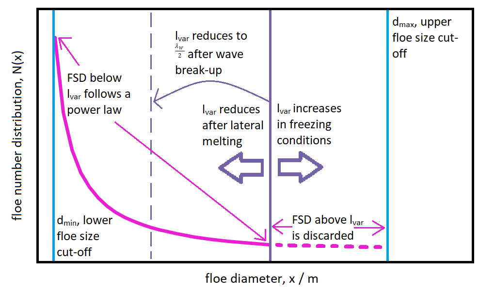
The Los Alamos sea ice model, hereafter referred to as CICE, usually assumes a fixed floe size of 300 m. We can impose a simple FSD model into CICE derived from a power law to explore the impact of variable floe size on the sea ice cover. Figure 1 is a diagram of the WIPoFSD model (Waves-in-Ice module and Power law Floe Size Distribution model), which assumes a power law with a fixed exponent, , between a lower floe size cut-off, , and an upper floe size cut-off, . The model also incorporates a floe size variable, , to capture the effects of processes that can influence floe size. The processes represented are wave break-up of floes, melting at the floe edge, winter floe growth, and advection. The model includes a wave advection and attenuation scheme so that wave properties can be determined within the sea ice field to enable the identification of wave break-up events. Full details of the WIPoFSD model and its implementation into CICE are available in Bateson et al. (2020). For the WIPoFSD model setup considered here, we explore the impact of the FSD on the lateral melt rate, which is the melt rate at the edge surfaces of floes. It is useful to define a new FSD metric that can be used to characterise the impact of the FSD on lateral melt. To do this we note that the lateral melt volume produced by a floe is proportional to the perimeter of the floe. The effective floe size, , is defined as a fixed floe size that would produce the same lateral melt rate as a given FSD, for a fixed total sea ice area.

Here we will compare a CICE simulation incorporating the WIPoFSD model, hereafter referred to as stan-fsd, to a reference case, ref, using the CICE standard fixed floe size of 300 m. For the WIPoFSD model, = 10 m, = 30 km, and = -2.5. These values have been selected as representative values from observations. The reference setup is initiated in 1990 and spun-up until 2005, when either continued as ref or the WIPoFSD model imposed for stan-fsd before being evaluated from 2006 – 2016. All figures in this post are given as a mean over 2007 – 2016, such that 2005 – 2006 is a period of spin-up for the incorporated WIPoFSD model.

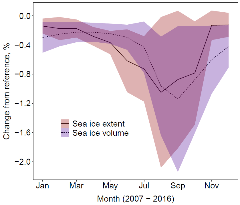
In Figure 2, we show the percentage reduction in the Arctic sea ice extent and volume of stan-fsd relative to ref. The differences in both extent and volume over the pan-Arctic scale evolve over an annual cycle, with maximum differences of -1.0 % in August and -1.1 % in September respectively. The annual cycle corresponds to periods of melting and freeze-up and is a product of the nature of the imposed FSD. Lateral melt rates are a function of floe size, but freeze-up rates are not, hence model differences only increase during periods of melting and not during periods of freeze-up. The difference in sea ice extent reduces rapidly during freeze-up because this freeze-up is predominantly driven by ocean surface properties, which are strongly coupled to atmospheric conditions in areas of low sea ice extent. In comparison, whilst atmospheric conditions initiate the vertical sea ice growth, this atmosphere-ocean coupling is rapidly lost due to insulation of the warmer ocean from the cooler atmosphere once sea ice extends across the horizontal plane. Hence a residual difference in sea ice thickness and therefore volume propagates throughout the winter season. The interannual variability shows that the impact of the WIPoFSD model with standard parameters varies significantly depending on the year.

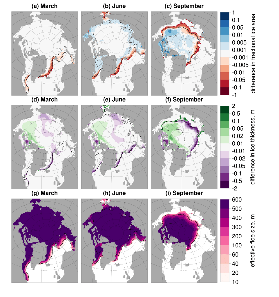
Although the pan-Arctic differences in extent and volume shown in Figure 2 are marginal, differences are larger when considering smaller spatial scales. Figure 3 shows the spatial distribution in the changes in sea ice concentration and thickness in March, June, and September for stan-fsd relative to ref in addition to the spatial distribution in for stan-fsd for the same months. Reductions in the sea ice concentration and thickness of up to 0.1 and 50 cm observed respectively in the September marginal ice zone (MIZ). Within the pack ice, increases in the sea ice concentration of up to 0.05 and ice thickness of up to 10 cm can be seen. To understand the non-uniform spatial impacts of the FSD, it is useful to look at the behaviour of . Regions with an greater than 300 m will experience less lateral melt than the equivalent location in ref (all other things being equal) whereas locations with an below 300 m will experience more lateral melt. In Figure 3 we see the transition to values of smaller than 300 m in the MIZ, hence most of the sea ice cover experiences less lateral melting for stan-fsd compared to ref.

For Figures 2-3, the parameters used to define the FSD have been set to fixed, standard values. However, these parameters vary significantly between different observed FSDs. It is therefore useful to explore the model sensitivity to these parameters. For α values of -2, -2.5, -3 and -3.5 have been selected to span the general range of values reported in observations (Stern et al., 2018a). For values of 1 m, 20 m and 50 m are selected to reflect the different behaviours reported in studies, with some showing power law behaviour extending to 1 m (Toyota et al., 2006) and others showing a tailing off at an order of 10 s of metres (Stern et al., 2018b). For the upper cut-off, , values of 1000 m, 10,000 m, 30,000 m and 50,000 m are selected, again to represent the distributions reported in different studies. 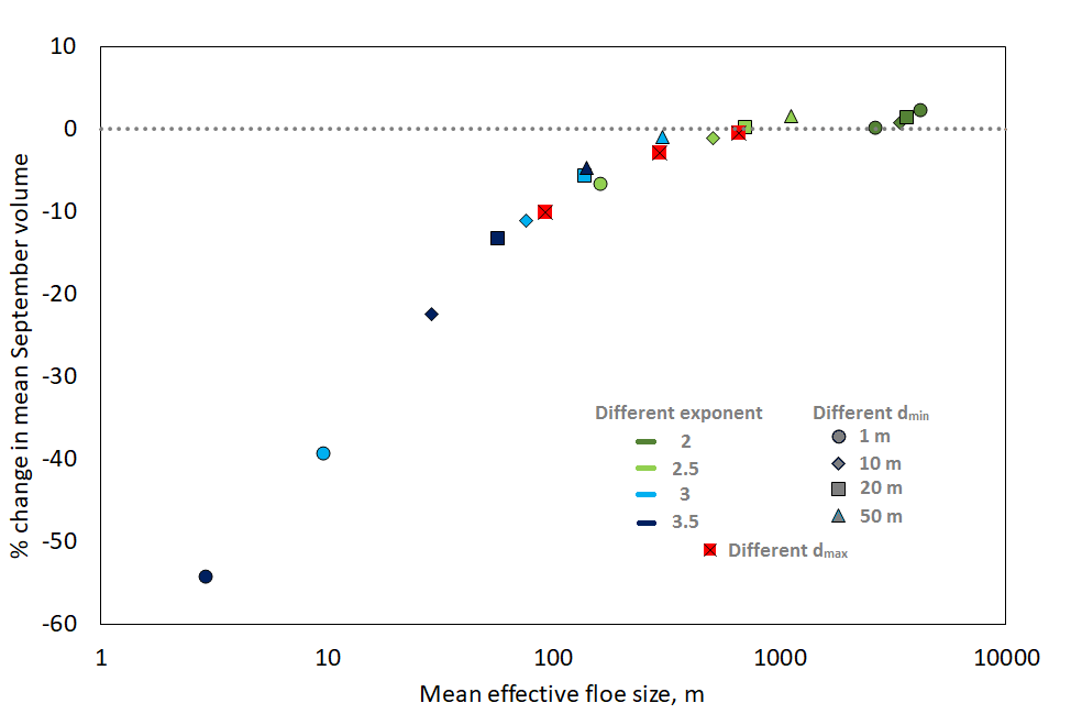50 km is taken as the largest value for as this serves as an upper limit to what can be resolved within an individual grid cell on a CICE 1 grid. A total of 19 sensitivity studies have been completed used different permutations of the stated values for the FSD model parameters. Figure 4 shows the change in mean September sea ice extent and volume relative to ref plotted against mean annual , averaged over the sea ice extent, for each of these sensitivity studies. The impacts range from a small increase in extent and volume to large reductions of -22 % and -55 % respectively, even within the parameter space defined by observations. Furthermore, there is almost a one-to-one mapping between mean and extent and volume reduction. This suggests is a useful diagnostic tool to predict the impact of a given set of floe size parameters. The system varies most in response to the changes in the α, but it is also particularly sensitive to .

There are several advantages to the assumption of a fixed power law in modelling the sea ice floe size distribution. It provides a simple framework to explore the potential impact of an observed FSD on the sea ice mass balance, given observations of the FSD are generally fitted to a power law. In addition, the use of a simple model makes it easier to constrain the mechanism of how the model changes the sea ice cover. However, there are also significant disadvantages including the high model sensitivity to poorly constrained parameters, as shown in Figure 4. In addition, there is evidence both that the exponent evolves over an annual cycle and is not a fixed value (Stern et al., 2018b) and that the power law is not a statistically valid description of the FSD over all floe sizes (Horvat et al., 2019). An alternative approach to modelling the FSD is the prognostic model of Roach et al. (2018, 2019). The prognostic model avoids any assumptions about the shape of the distribution and instead assigns sea ice area to a set of adjacent floe size categories, with individual processes parameterised at floe scale. This approach carries its own set of challenges. If important physical processes are missing from the model it will not be possible to simulate a physically realistic distribution. In addition, the prognostic model has a significant computational cost. In practice, the choice of FSD modelling approach will depend on the application.

Further reading
Bateson, A. W., Feltham, D. L., Schröder, D., Hosekova, L., Ridley, J. K. and Aksenov, Y.: Impact of sea ice floe size distribution on seasonal fragmentation and melt of Arctic sea ice, Cryosphere, 14, 403–428, https://doi.org/10.5194/tc-14-403-2020, 2020.

Horvat, C., Roach, L. A., Tilling, R., Bitz, C. M., Fox-Kemper, B., Guider, C., Hill, K., Ridout, A., and Shepherd, A.: Estimating the sea ice floe size distribution using satellite altimetry: theory, climatology, and model comparison, The Cryosphere, 13, 2869–2885, https://doi.org/10.5194/tc-13-2869-2019, 2019. 

Stern, H. L., Schweiger, A. J., Zhang, J., and Steele, M.: On reconciling disparate studies of the sea-ice floe size distribution, Elem. Sci. Anth., 6, p. 49, https://doi.org/10.1525/elementa.304, 2018a. 

Stern, H. L., Schweiger, A. J., Stark, M., Zhang, J., Steele, M., and Hwang, B.: Seasonal evolution of the sea-ice floe size distribution in the Beaufort and Chukchi seas, Elem. Sci. Anth., 6, p. 48, https://doi.org/10.1525/elementa.305, 2018b. 

Roach, L. A., Horvat, C., Dean, S. M., and Bitz, C. M.: An Emergent Sea Ice Floe Size Distribution in a Global Coupled Ocean-Sea Ice Model, J. Geophys. Res.-Oceans, 123, 4322–4337, https://doi.org/10.1029/2017JC013692, 2018. 

Roach, L. A., Bitz, C. M., Horvat, C. and Dean, S. M.: Advances in Modeling Interactions Between Sea Ice and Ocean Surface Waves, J. Adv. Model. Earth Syst., 11, 4167–4181, https://doi.org/10.1029/2019MS001836, 2019.

Toyota, T., Takatsuji, S., and Nakayama, M.: Characteristics of sea ice floe size distribution in the seasonal ice zone, Geophys. Res. Lett., 33, 2–5, https://doi.org/10.1029/2005GL024556, 2006.