Arctic Summer-time Cyclones Field Campaign in Svalbard

Hannah Croad – h.croad@pgr.reading.ac.uk

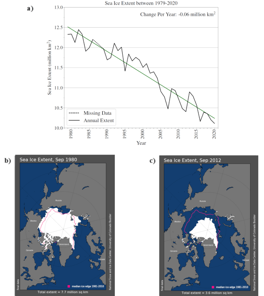
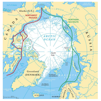
The rapid decline of sea ice is permitting increased human activity in the summer-time Arctic, where it will be exposed to the risks of Arctic weather. Arctic cyclones are the major weather hazard in the summer-time Arctic, producing strong winds and ocean waves that impact sea ice over large areas. My PhD project is about understanding the dynamics of Arctic summer-time cyclones. One of the biggest uncertainties in our understanding is the interaction of cyclones with the surface and sea ice. Sea ice-atmosphere coupling is greatest in summer when the ice is thinner and more mobile. Strong winds associated with cyclones can move and alter the sea ice, but the sea ice state also feeds back on the development of cyclones, determining surface drag and turbulent fluxes of heat and moisture


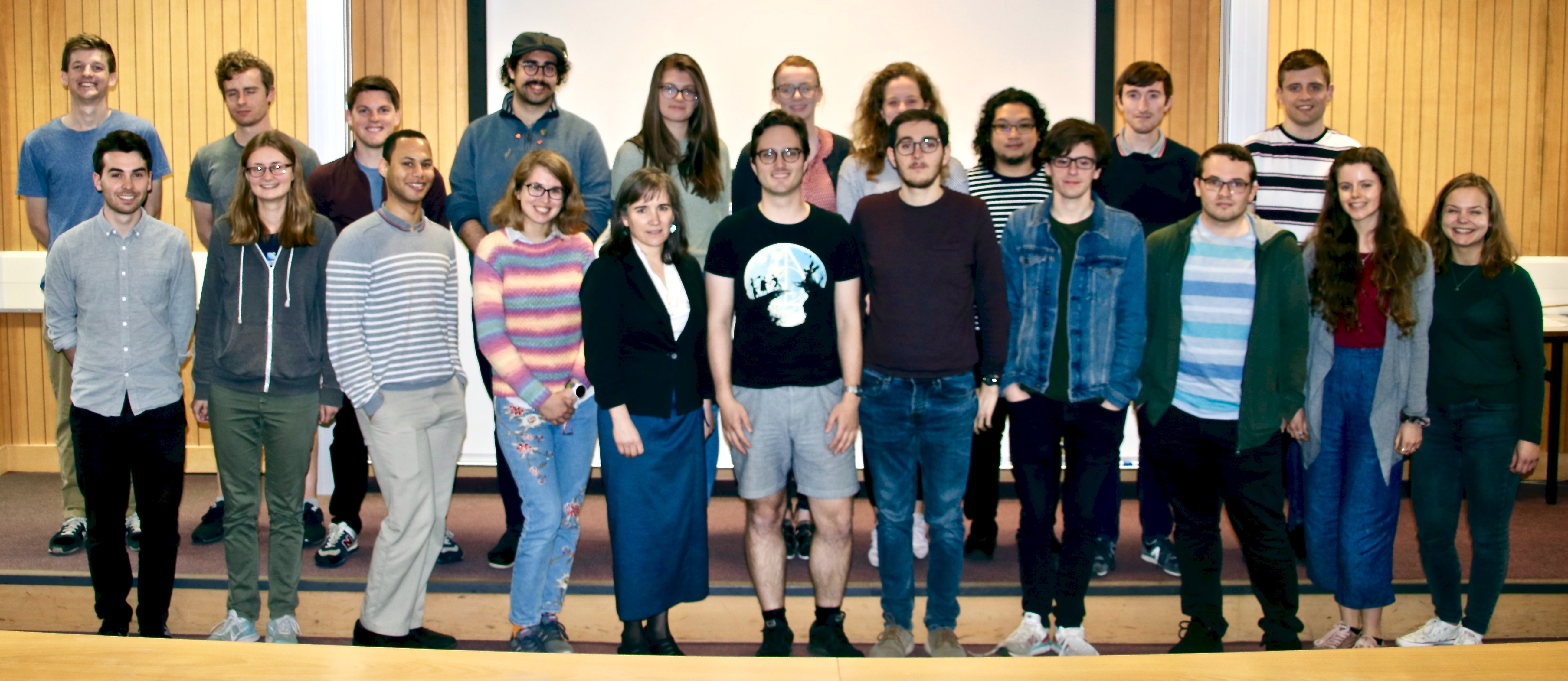
My PhD project is closely linked with the Arctic Summer-time Cyclones NERC project, and therefore, I had the opportunity to join the associated field campaign. The field campaign team is comprised of scientists, engineers and pilots from the University of Reading, the University of East Anglia and British Antarctic Survey (BAS). The primary aim of the field campaign was to fly through Arctic cyclones, (i) mapping cyclone structure and (ii) obtaining measurements necessary to characterise the cyclone-sea interaction. In particular, observations of near-surface fluxes of momentum, heat and moisture over sea ice and ocean are needed, as these fluxes dictate the impact of the surface on cyclones. These observations are needed to evaluate and improve the representation of turbulent exchange in numerical weather prediction (NWP) models, especially over sea ice where there are not many existing observations. To obtain accurate measurements of near-surface fluxes, we need to be quite close to the surface (no higher than 300 ft). To do this, we would be using BAS’s Twin Otter aircraft, equipped with Meteorological Airborne Science INstrumentation (MASIN). The twin-engine prop aircraft is small and light, and is therefore ideal for flying at low-levels just above the surface (as low as 50 ft!). There are many instruments fitted on the MASIN research aircraft, but the most important measurements for our purposes were temperature, wind speed, humidity (important for mapping cyclone structure), surface layer turbulent fluxes (from the 50 Hz turbulence probe), and ice surface properties (from laser altimeter).

British Antarctic Survey’s Twin Otter aircraft, fitted with the MASIN equipment. You can see the turbulence probe on the boom at the front of the aircraft, and the CAPS (cloud, aerosol, and precipitation spectrometer) probe on the left wing. The pilot is on top of the aircraft, carrying out final checks before a science flight. Photo from John Methven.

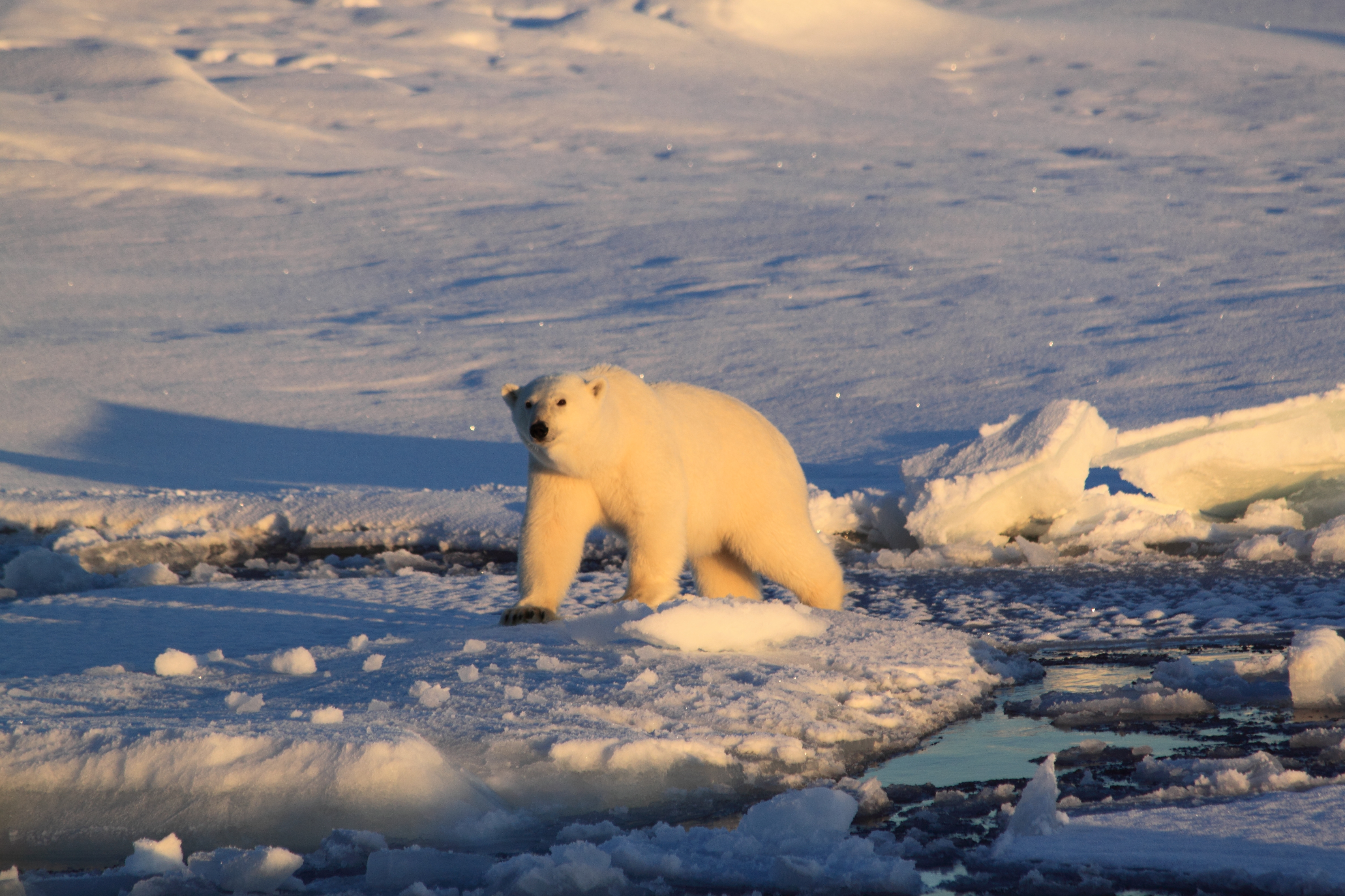
After a 1-year delay due to the Covid-19 pandemic, the field campaign took place in July and August 2022. We were based on the Norwegian archipelago of Svalbard, a 3-hour flight north of Oslo. The team was based in Longyearbyen, the main town on Svalbard. At 78°N, Svalbard is the most northern town in the world! Longyearbyen is located within a valley on the shore of Adventfjorden. The town is a strange but charming place with lots of eccentricities. Longyearbyen is populated with wooden buildings, with pipes above the ground (as the ground freezes in winter), and old mining structures on the sides of the valley. The town is small, but well provided for, with a few tourist shops, restaurants, and a supermarket. As Svalbard is in the Arctic circle, during the summer months it experiences 24-hour sunlight, which was very strange! Furthermore, Longyearbyen is one of the only places on Svalbard that is ‘polar bear safe’ – you should only leave the town limits if you have a rifle!


The field campaign team worked at Longyearbyen airport. The team would study the forecasts from different weather models for the next week, to decide on flight plans. We were primarily looking for strong winds (ideally associated with cyclones, but beggars can’t be choosers!) over the sea ice, within range of the Twin Otter aircraft (approximately 600 nautical miles). With flight planning, there were many things to consider. It was a case of waiting for good weather to come to us, and planning rest days for the pilots when the weather wasn’t looking so interesting in the forecast. Flight plans would consist of transit to and from the target region, where science would be conducted. Science flying included low-level legs to obtain turbulent flux measurements, vertical profiles of the boundary layer, and stacked cross-sections through cyclone features (e.g. fronts) in and above the boundary layer. For flights where low-level flying was planned, it was key that there should not be low cloud in the target area, as this would prevent the aircraft from flying below 1000 ft for safety reasons. It was also important that there were no bad conditions (poor visibility or strong winds) in Longyearbyen, which would prevent the aircraft from taking off or landing. Longyearbyen is an isolated airfield, and the aircraft cannot carry enough fuel to make it back to the mainland if conditions are too poor to land, so this was a very important consideration. Furthermore, the American and French THINICE project field campaign was being conducted at the same time in Svalbard, with the SAFIRE ATR42 aircraft flying at higher levels, looking downwards on Arctic cyclones. We were able to co-ordinate several flights through the same weather systems, with the Twin Otter aircraft flying below the ATR42.


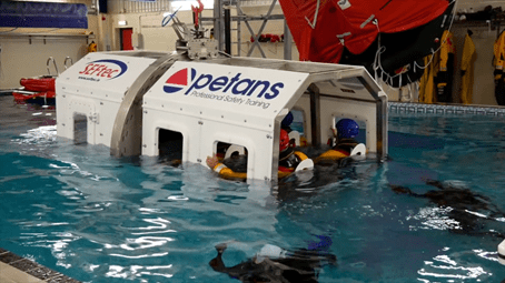
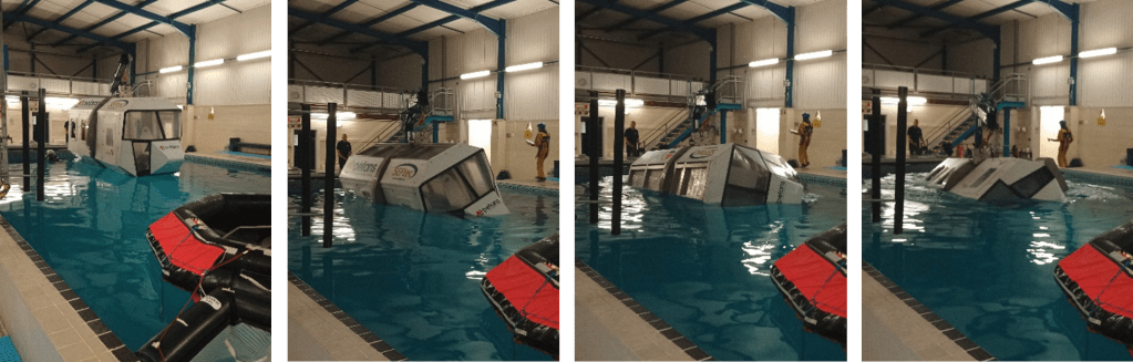
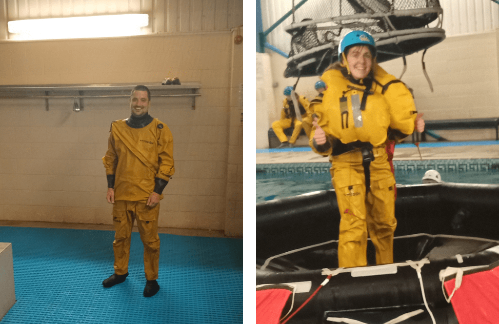
The Twin Otter aircraft holds 3-4 people, including the pilot. With an instrument engineer also on board, this left space for 1 or 2 scientists on each flight (Note: to fly on the aircraft we had to do helicopter underwater escape training – see my previous blog at https://socialmetwork.blog/2021/07/16/helicopter-underwater-escape-training-for-arctic-field-campaign/). The cabin is very small (too small for a person to stand up), and is rather cramped, with a considerable amount of space taken up by the extra range fuel tank! The aircraft is flown between 50 and 10,000 ft, and so the cabin is not pressurized. For low-level flying, the crew must wear immersion suits and life jackets on the aircraft (in the unlikely event that the aircraft must ditch in the ocean). On the flight the crew wear noise-cancelling headphones (as the engines are rather loud), and everyone can speak to each other over the intercom. During the flight the scientists will alter the flight plan if necessary, depending on the conditions they encounter, and take notes of the environment and any notable events that occur during the flight. This includes noting what they can see out of the window (e.g. sea ice fraction, cloud), any interesting observations from the live feed of the instrument output within the aircraft (e.g. boundary layer depth), and any instruments that are not working or faulty.


I had the opportunity to fly on the aircraft on the third science flight of the field campaign (I wrote about this in another blog: https://research.reading.ac.uk/arctic-summertime-cyclones/first-field-campaign-flying-experience/). We were targeting a region to the north-west of Svalbard, in the Fram Strait, where there was forecast to be strong northerly winds over the marginal ice zone. The primary objective was to measure turbulent fluxes over sea ice at low-level. However, on reaching the target region, we were unable to descend lower than 500 ft due to cloud and Arctic sea smoke (formed as cold Arctic air moves over warmer water in between the sea ice floes) at the surface – not safe conditions for flying at low-level! Through gaps in the clouds, we got a glimpse at the Arctic sea smoke over the marginal ice zone (see below). (Note: Several other flights in the field campaign encountered better conditions and were able to get to low levels – see video below!). We searched for better conditions near the target region for an hour, but didn’t find any, so made the return trip home. It was a shame that we could not fly low enough to obtain turbulent flux measurements, but the flight was still useful for obtaining profiles of wind structure in the boundary layer, and for our understanding of forecast performance in the region.

Photos taken from the Twin Otter aircraft 500 ft above the surface, with a layer of Arctic sea smoke overlaying the ice floes of the marginal ice zone. Here visibility is too low to descend any further. Photos from Hannah Croad.
Flying over the marginal ice zone at 70 ft in good visibility conditions, with the shadow of the Twin Otter aircraft visible. Video from John Methven.

During the month-long field campaign a total of 17 science flights were conducted, flying in all directions from Longyearbyen, with an accumulated 80 hours of flying time. This included 4 Arctic cyclone cases, and 7.5 hours of surface layer turbulent flux measurements (more than we could have hoped for!). The data from the aircraft is currently undergoing quality control. Analysis will now proceed in two streams:

  1. Run simulations of Arctic cyclone cases in NWP models, evaluating against field campaign observations and using various tools to relate surface friction and heating to cyclone evolution (led by the University of Reading team)
  2. Use observations of turbulent fluxes in the surface layer over the marginal ice zone and sea ice properties to improve the representation of turbulent exchange over sea ice – i.e. develop parametrizations (led by the University of East Anglia team)

Building on the outputs and findings from these two work packages, we will then run sensitivity experiments of Arctic cyclones in NWP models, using the revised turbulent exchange parametrizations, to understand the impact on cyclone development.

A summary of all the science flights conducted during the Arctic Summer-time Cyclones field campaign. Flight routes are coloured blue-yellow, indicating flight altitude. Also plotted is the campaign mean sea ice fraction (AMSR2).

I really enjoyed my time on the field campaign, and I learnt a lot! It was great to help the team with forecasting and flight planning, and to be on a science flight. I also got to do a bit of media work, talking on BBC Radio 4’s Inside Science programme (https://www.bbc.co.uk/programmes/m0019z2y). It was a fantastic experience, and now the team and I are looking forward to getting started with the analysis and using the data!

Arctic Summer-time Cyclones field campaign team (some missing) in front of the Twin Otter aircraft. Photo from Dan Beeden.

Helicopter Underwater Escape Training for Arctic Field Campaign

Hannah Croad h.croad@pgr.reading.ac.uk

The focus of my PhD project is investigating the physical mechanisms behind the growth and evolution of summer-time Arctic cyclones, including the interaction between cyclones and sea ice. The rapid decline of Arctic sea ice extent is allowing human activity (e.g. shipping) to expand into the summer-time Arctic, where it will be exposed to the risks of Arctic weather. Arctic cyclones produce some of the most impactful Arctic weather, associated with strong winds and atmospheric forcings that have large impacts on the sea ice. Hence, there is a demand for improved forecasts, which can be achieved through a better understanding of Arctic cyclone mechanisms. 

My PhD project is closely linked with a NERC project (Arctic Summer-time Cyclones: Dynamics and Sea-ice Interaction), with an associated field campaign. Whereas my PhD project is focused on Arctic cyclone mechanisms, the primary aims of the NERC project are to understand the influence of sea ice conditions on summer-time Arctic cyclone development, and the interaction of cyclones with the summer-time Arctic environment. The field campaign, originally planned for August 2021 based in Svalbard in the Norwegian Arctic, has now been postponed to August 2022 (due to ongoing restrictions on international travel and associated risks for research operations due to the evolving Covid pandemic). The field campaign will use the British Antarctic Survey’s low-flying Twin Otter aircraft, equipped with infrared and lidar instruments, to take measurements of near-surface fluxes of momentum, heat and moisture associated with cyclones over sea ice and the neighbouring ocean. These simultaneous observations of turbulent fluxes in the atmospheric boundary layer and sea ice characteristics, in the vicinity of Arctic cyclones, are needed to improve the representation of turbulent exchange over sea ice in numerical weather prediction models. 

Those wishing to fly onboard the Twin Otter research aircraft are required to do Helicopter Underwater Escape Training (HUET). Most of the participants on the course travel to and from offshore facilities, as the course is compulsory for all passengers on the helicopters to rigs. In the unlikely event that a helicopter must ditch on the ocean, although the aircraft has buoyancy aids, capsize is likely because the engine and rotors make the aircraft top heavy. I was apprehensive about doing the training, as having to escape from a submerged aircraft is not exactly my idea of fun. However, I realise that being able to fly on the research aircraft in the Arctic is a unique opportunity, so I was willing to take on the challenge! 

The HUET course is provided by the Petans training facility in Norwich. John Methven, Ben Harvey, and I drove to Norwich the night before, in preparation for an early start the next day. We spent the morning in the classroom, covering helicopter escape procedures and what we should expect for the practical session in the afternoon. We would have to escape from a simulator recreating a crash landing on water. The simulator replicates a helicopter fuselage, with seats and windows, attached to the end of a mechanical arm for controlled submersion and rotation. The procedure is (i) prepare for emergency landing: check seatbelt is pulled tight, headgear is on, and that all loose objects are tucked away, (ii) assume the brace position on impact, and (iii) keep one hand on the window exit and the other on your seatbelt buckle. Once submerged, undo your seatbelt and escape through the window. After a nervy lunch, it was time to put this into practice. 

The aircraft simulator being submerged in the pool (Source: Petans promotional video

The practical part of the course took place in a pool (the temperature resembled lukewarm bath water, much warmer than the North Atlantic!). We were kitted up with two sets of overalls over our swimming costumes, shoes, helmets, and jackets containing a buoyancy aid. We then began the training in the aircraft simulator. Climb into the aircraft and strap yourself into a seat. The seatbelt had to be pulled tight, and was released by rotating the central buckle. On the pilots command, prepare for emergency landing. Assume the brace position, and the aircraft drops into the water. Hold on to the window and your seatbelt buckle, and as the water reaches your chest, take a deep breath. Wait for the cabin to completely fill with water and stop moving – only then undo your seatbelt and get out! 

The practical session consisted of three parts. In the first exercise, the aircraft was submerged, and you had to escape through the window. The second exercise was similar, except that panes were fitted on the windows, which you had to push out before escaping. In the final exercise, the aircraft was submerged and rotated 180 degrees, so you ended up upside down (and with plenty of water up your nose), which was very disorientating! Each exercise required you to hold your breath for roughly 10 seconds at a time. Once we had escaped and reached the surface, we deployed our buoyancy aids, and climbed to safety onto the life raft. 

Going for a spin! The aircraft simulator being rotated with me strapped in
Ben and I happy to have survived the training!

The experience was nerve-wracking, and really forced me to push myself out of my comfort zone. I didn’t need to be too worried though, even after struggling with undoing the seatbelt a couple of times, I was assisted by the diving team and encouraged to go again. I was glad to get through the exercises, and pass the course along with the others. This was an amazing experience (definitely not something I expected to do when applying for a PhD!), and I’m now looking forward to the field campaign next year. 

Quantifying Arctic Storm Risk in a Changing Climate

Alec Vessey (Final Year PhD Student) – alexandervessey@pgr.reading.ac.uk 
Supervisors: Kevin Hodges (UoR), Len Shaffrey (UoR), Jonny Day (ECMWF), John Wardman (AXA XL)
 

Arctic sea ice extent has reduced dramatically since it was first monitored by satellites in 1979 – at a rate of 60,000 km2 per year (see Figure 1a). This is equivalent to losing an ice sheet the size of London every 10 days. This dramatic reduction in sea ice extent has been caused by global temperatures increasing, which is a result of anthropogenic climate change. The Arctic is the region of Earth that has undergone the greatest warming in recent decades, due to the positive feedback mechanism of Arctic Amplification. Global temperatures are expected to continue to increase into the 21st century, further reducing Arctic sea ice extent. 

Consequently, the Arctic Ocean has become increasingly open and navigable for ships (see Figure 1b and 1c). The Arctic Ocean provides shorter distances between ports in Europe and North America to ports in Asia than more traditional routes in the mid-latitudes that include the Suez Canal Route and the routes through the Panama Canal. There are two main shipping routes in the Arctic, the Northern Sea Route (along the coastline of Eurasia) and the Northwest Passage (through the Canadian Archipelago) (see Figure 2). For example, the distance between the Ports of Rotterdam and Tokyo can be reduced by 4,300 nautical-miles if ships travel through the Arctic (total distance: 7,000 nautical-miles) rather than using the mid-latitude route through the Suez Canal (total distance: 11,300 nautical-miles). Travelling through the Arctic could increase profits for shipping companies. Shorter journeys will require less fuel to be spent on between destinations and allow more time for additional shipping contracts to be pursued. It is expected that the number of ships in the Arctic will increase exponentially in the near future, when infrastructure is developed, and sea ice extent reduces further.  

Figure 1. Reductions in Arctic sea ice extent from 1979 – 2020. a) Annual Arctic sea ice extent per year between 1979-2020. b) Spatial distribution of Arctic sea ice in September 1980. c) Spatial distribution of Arctic sea ice in September 2012 (the lowest sea ice extent on record). Sourced from the National Sea and Ice Data Center.
Figure 2. A map of the two main shipping routes through the Arctic. The Northwest Passage connects North America with the Bering Strait (and onto Asia), and the Northern Sea Route connects Europe with the Bering Strait (and onto Asia). Source: BBC (2016).

However, as human activity in the Arctic increases, the vulnerability of valuable assets and the risk to life due to exposure to hazardous weather conditions also increases.  Hazardous weather conditions often occur during the passage of storms.  Storms cause high surface wind speeds and high ocean waves. Arctic storms have also been shown to lead to enhanced break up of sea ice, resulting in additional hazards when ice drifts towards shipping lanes. Furthermore, the Arctic environment is extremely cold, with search and rescue and other support infrastructure poorly established. Thus, the Arctic is a very challenging environment for human activity. 

Over the last century, the risks of mid-latitude storms and hurricanes have been a focal-point of research in the scientific community, due to their damaging impact in densely populated areas. Population in the Arctic has only just started to increase. It was only in 2008 that sea ice had retreated far enough for both of the Arctic shipping lanes to be open simultaneously (European Space Agency, 2008). Arctic storms are less well understood than these hazards, mainly because they have not been a primary focus of research. Reductions in sea ice extent and increasing human activity mean that it is imperative to further the understanding of Arctic storms. 

This is what my PhD project is all about – quantifying the risk of Arctic storms in a changing climate. My project has four main questions, which try to fill the research gaps surrounding Arctic storm risk. These questions include: 

  1. What are the present characteristics (frequency, spatial distribution, intensity) of Arctic storms, and, what is the associated uncertainty of this when using different datasets and storm tracking algorithms? 
  1. What is the structure and development of Arctic storms, and how does this differ to that of mid-latitude storms? 
  1. How might Arctic storms change in a future climate in response to climate change? 
  1. Can the risk of Arctic storms impacting shipping activities be quantified by combining storm track data and ship track data? 

Results of my first research question are summarised in a recent paper (https://link.springer.com/article/10.1007/s00382-020-05142-4 – Vessey et al. 2020).  I previously wrote a blog post on the The Social Metwork summarising this paper, which can be found at https://socialmetwork.blog/2020/02/21/arctic-storms-in-multiple-global-reanalysis-datasets/. This showed that there is a seasonality to Arctic storms, with most winter (DJF) Arctic storms occurring in the Greenland, Norwegian and Barents Sea region, whereas, summer (JJA) Arctic storms generally occur over the coastline of Eurasia and the high Arctic Ocean. Despite the dramatic reductions in Arctic sea ice over the past few decades (see Figure 1), there is no trend in Arctic storm frequency. In the paper, the uncertainty in the present climate characteristics of Arctic storms is assessed, by using multiple reanalysis datasets and tracking methods. A reanalysis datasets is our best approximation of past atmospheric conditions, that combines past observations with state-of-the-art Numerical Weather Prediction Models. 

The deadline for my PhD project is the 30th of June 2021, so I am currently experiencing the very busy period of writing up my Thesis. Hopefully, there aren’t too many hiccups over the next few months, and perhaps I will be able to write some of my research chapters up as papers.  

References: 

BBC, 2016, Arctic Ocean shipping routes ‘to open for months’. https://www.bbc.com/news/science-environment-37286750. Accessed 18 March 2021. 

European Space Agency, 2008: Arctic sea ice annual freeze-up underway. https://www.esa.int/Applications/Observing_the_Earth/Space_for_our_climate/Arctic_sea_ice_annual_freeze_nobr_-up_nobr_underway. Accessed 18 March 2021. 

National Snow & Ice Data Centre, (2021), Sea Ice Index. https://nsidc.org/data/seaice_index. Accessed 18 March 2021. 

Vessey, A.F., K.I., Hodges, L.C., Shaffrey and J.J. Day, 2020: An Inter-comparison of Arctic synoptic scale storms between four global reanalysis datasets. Climate Dynamics, 54 (5), 2777-2795. 

Exploring the impact of variable floe size on the Arctic sea ice

Email: a.w.bateson@pgr.reading.ac.uk

The Arctic sea ice cover is made up of discrete units of sea ice area called floes. The size of these floes has an impact on several sea ice processes including the volume of melt produced at floe edges, the momentum exchange between the sea ice, ocean, and atmosphere, and the mechanical response of the sea ice to stress. Models of the sea ice have traditionally assumed that floes adopt a uniform size, if floe size is explicitly represented at all in the model. Observations of floes show that floe size can span a huge range, from scales of metres to tens of kilometres. Generally, observations of the floe size distribution (FSD) are fitted to a power law or a combination of power laws (Stern et al., 2018a).

The Los Alamos sea ice model, hereafter referred to as CICE, usually assumes a fixed floe size of 300 m. We can impose a simple FSD model into CICE derived from a power law to explore the impact of variable floe size on the sea ice cover. Figure 1 is a diagram of the WIPoFSD model (Waves-in-Ice module and Power law Floe Size Distribution model), which assumes a power law with a fixed exponent, \alpha, between a lower floe size cut-off, d_{min}, and an upper floe size cut-off, d_{max}. The model also incorporates a floe size variable, l_{var}, to capture the effects of processes that can influence floe size. The processes represented are wave break-up of floes, melting at the floe edge, winter floe growth, and advection. The model includes a wave advection and attenuation scheme so that wave properties can be determined within the sea ice field to enable the identification of wave break-up events. Full details of the WIPoFSD model and its implementation into CICE are available in Bateson et al. (2020). For the WIPoFSD model setup considered here, we explore the impact of the FSD on the lateral melt rate, which is the melt rate at the edge surfaces of floes. It is useful to define a new FSD metric that can be used to characterise the impact of the FSD on lateral melt. To do this we note that the lateral melt volume produced by a floe is proportional to the perimeter of the floe. The effective floe size, l_{eff}, is defined as a fixed floe size that would produce the same lateral melt rate as a given FSD, for a fixed total sea ice area.

Figure 1: A schematic of the imposed FSD model. This model is initiated by prescribing a power law with an exponent, \alpha, and between the limits d_{min} and d_{max}. Within individual grid cells the variable FSD tracer, l_{var}, varies between these two limits. l_{var} evolves through lateral melting, wave break-up events, freezing, and advection.

Here we will compare a CICE simulation incorporating the WIPoFSD model, hereafter referred to as stan-fsd, to a reference case, ref, using the CICE standard fixed floe size of 300 m. For the WIPoFSD model, d_{min} = 10 m, d_{max} = 30 km, and \alpha = -2.5. These values have been selected as representative values from observations. The reference setup is initiated in 1990 and spun-up until 2005, when either continued as ref or the WIPoFSD model imposed for stan-fsd before being evaluated from 2006 – 2016. All figures in this post are given as a mean over 2007 – 2016, such that 2005 – 2006 is a period of spin-up for the incorporated WIPoFSD model.

In Figure 2, we show the percentage reduction in the Arctic sea ice extent and volume of stan-fsd relative to ref. The differences in both extent and volume over the pan-Arctic scale evolve over an annual cycle, with maximum differences of -1.0 % in August and -1.1 % in September respectively. The annual cycle corresponds to periods of melting and freeze-up and is a product of the nature of the imposed FSD. Lateral melt rates are a function of floe size, but freeze-up rates are not, hence model differences only increase during periods of melting and not during periods of freeze-up. The difference in sea ice extent reduces rapidly during freeze-up because this freeze-up is predominantly driven by ocean surface properties, which are strongly coupled to atmospheric conditions in areas of low sea ice extent. In comparison, whilst atmospheric conditions initiate the vertical sea ice growth, this atmosphere-ocean coupling is rapidly lost due to insulation of the warmer ocean from the cooler atmosphere once sea ice extends across the horizontal plane. Hence a residual difference in sea ice thickness and therefore volume propagates throughout the winter season. The interannual variability shows that the impact of the WIPoFSD model with standard parameters varies significantly depending on the year.

Figure 2: Difference in sea ice extent (solid, red ribbon) and volume (dashed, blue ribbon) between stan-fsd relative to ref averaged over 2007–2016. The ribbon shows the region spanned by the mean value plus or minus 2 times the standard deviation for each simulation. This gives a measure of the interannual variability over the 10-year period.

Although the pan-Arctic differences in extent and volume shown in Figure 2 are marginal, differences are larger when considering smaller spatial scales. Figure 3 shows the spatial distribution in the changes in sea ice concentration and thickness in March, June, and September for stan-fsd relative to ref in addition to the spatial distribution in l_{eff} for stan-fsd for the same months. Reductions in the sea ice concentration and thickness of up to 0.1 and 50 cm observed respectively in the September marginal ice zone (MIZ). Within the pack ice, increases in the sea ice concentration of up to 0.05 and ice thickness of up to 10 cm can be seen. To understand the non-uniform spatial impacts of the FSD, it is useful to look at the behaviour of l_{eff}. Regions with an l_{eff} greater than 300 m will experience less lateral melt than the equivalent location in ref (all other things being equal) whereas locations with an l_{eff} below 300 m will experience more lateral melt. In Figure 3 we see the transition to values of l_{eff} smaller than 300 m in the MIZ, hence most of the sea ice cover experiences less lateral melting for stan-fsd compared to ref.

Figure 3: Difference in the sea ice concentration (top row, a-c) and thickness (middle row, d-f) between stan-fsd and ref and l_{eff} (bottom row, g-i) for stan-fsd averaged over 2007 – 2016. Results are presented for March (left column, a, d, g), June (middle column, b, e, h) and September (right column, c, f, i). Values are shown only in locations where the sea ice concentration exceeds 5 %.

For Figures 2-3, the parameters used to define the FSD have been set to fixed, standard values. However, these parameters vary significantly between different observed FSDs. It is therefore useful to explore the model sensitivity to these parameters. For α values of -2, -2.5, -3 and -3.5 have been selected to span the general range of values reported in observations (Stern et al., 2018a). For d_{min} values of 1 m, 20 m and 50 m are selected to reflect the different behaviours reported in studies, with some showing power law behaviour extending to 1 m (Toyota et al., 2006) and others showing a tailing off at an order of 10 s of metres (Stern et al., 2018b). For the upper cut-off, d_{max}, values of 1000 m, 10,000 m, 30,000 m and 50,000 m are selected, again to represent the distributions reported in different studies. 50 km is taken as the largest value for d_{max} as this serves as an upper limit to what can be resolved within an individual grid cell on a CICE 1^{\circ} 
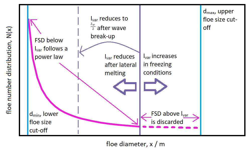
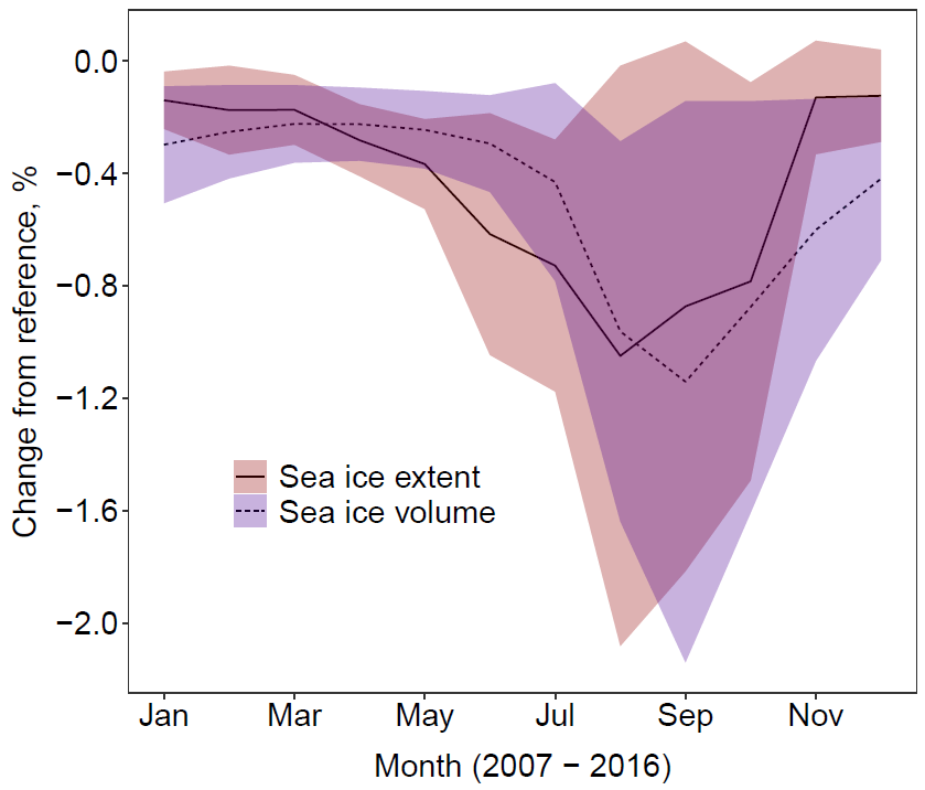
grid. A total of 19 sensitivity studies have been completed used different permutations of the stated values for the FSD model parameters. Figure 4 shows the change in mean September sea ice extent and volume relative to ref plotted against mean annual l_{eff}, averaged over the sea ice extent, for each of these sensitivity studies. The impacts range from a small increase in extent and volume to large reductions of -22 % and -55 % respectively, even within the parameter space defined by observations. Furthermore, there is almost a one-to-one mapping between mean l_{eff} and extent and volume reduction. This suggests l_{eff} is a useful diagnostic tool to predict the impact of a given set of floe size parameters. The system varies most in response to the changes in the α, but it is also particularly sensitive to d_{min}.

Figure 4: Relative change (%) in mean September sea ice volume from 2007 – 2016 respectively, plotted against mean l_{eff} for simulations with different selections of parameters relative to ref. The mean l_{eff} is taken as the equally weighted average across all grid cells where the sea ice concentration exceeds 15%. The colour of the marker indicates the value of the \alpha, the shape indicates the value of d_{min}, and the three experiments using standard parameters but different d_{max} (1000 m, 10000 m and 50000 m) are indicated by a crossed red square. The parameters are selected to be representative of a parameter space for the WIPoFSD model that has been constrained by observations.

There are several advantages to the assumption of a fixed power law in modelling the sea ice floe size distribution. It provides a simple framework to explore the potential impact of an observed FSD on the sea ice mass balance, given observations of the FSD are generally fitted to a power law. In addition, the use of a simple model makes it easier to constrain the mechanism of how the model changes the sea ice cover. However, there are also significant disadvantages including the high model sensitivity to poorly constrained parameters, as shown in Figure 4. In addition, there is evidence both that the exponent evolves over an annual cycle and is not a fixed value (Stern et al., 2018b) and that the power law is not a statistically valid description of the FSD over all floe sizes (Horvat et al., 2019). An alternative approach to modelling the FSD is the prognostic model of Roach et al. (2018, 2019). The prognostic model avoids any assumptions about the shape of the distribution and instead assigns sea ice area to a set of adjacent floe size categories, with individual processes parameterised at floe scale. This approach carries its own set of challenges. If important physical processes are missing from the model it will not be possible to simulate a physically realistic distribution. In addition, the prognostic model has a significant computational cost. In practice, the choice of FSD modelling approach will depend on the application.

Further reading
Bateson, A. W., Feltham, D. L., Schröder, D., Hosekova, L., Ridley, J. K. and Aksenov, Y.: Impact of sea ice floe size distribution on seasonal fragmentation and melt of Arctic sea ice, Cryosphere, 14, 403–428, https://doi.org/10.5194/tc-14-403-2020, 2020.

Horvat, C., Roach, L. A., Tilling, R., Bitz, C. M., Fox-Kemper, B., Guider, C., Hill, K., Ridout, A., and Shepherd, A.: Estimating the sea ice floe size distribution using satellite altimetry: theory, climatology, and model comparison, The Cryosphere, 13, 2869–2885, https://doi.org/10.5194/tc-13-2869-2019, 2019. 

Stern, H. L., Schweiger, A. J., Zhang, J., and Steele, M.: On reconciling disparate studies of the sea-ice floe size distribution, Elem. Sci. Anth., 6, p. 49, https://doi.org/10.1525/elementa.304, 2018a. 

Stern, H. L., Schweiger, A. J., Stark, M., Zhang, J., Steele, M., and Hwang, B.: Seasonal evolution of the sea-ice floe size distribution in the Beaufort and Chukchi seas, Elem. Sci. Anth., 6, p. 48, https://doi.org/10.1525/elementa.305, 2018b. 

Roach, L. A., Horvat, C., Dean, S. M., and Bitz, C. M.: An Emergent Sea Ice Floe Size Distribution in a Global Coupled Ocean-Sea Ice Model, J. Geophys. Res.-Oceans, 123, 4322–4337, https://doi.org/10.1029/2017JC013692, 2018. 

Roach, L. A., Bitz, C. M., Horvat, C. and Dean, S. M.: Advances in Modeling Interactions Between Sea Ice and Ocean Surface Waves, J. Adv. Model. Earth Syst., 11, 4167–4181, https://doi.org/10.1029/2019MS001836, 2019.

Toyota, T., Takatsuji, S., and Nakayama, M.: Characteristics of sea ice floe size distribution in the seasonal ice zone, Geophys. Res. Lett., 33, 2–5, https://doi.org/10.1029/2005GL024556, 2006. 

How do ocean and atmospheric heat transports affect sea-ice extent?

Email: j.r.aylmer@pgr.reading.ac.uk

Downward trends in Arctic sea-ice extent in recent decades are a striking signal of our warming planet. Loss of sea ice has major implications for future climate because it strongly influences the Earth’s energy budget and plays a dynamic role in the atmosphere and ocean circulation.

Comprehensive numerical models are used to make long-term projections of the future climate state under different greenhouse gas emission scenarios. They estimate that the Arctic ocean will become seasonally ice free by the end of the 21st century, but there is a large uncertainty on the timing due to the spread of estimates across models (Fig. 1).

Figure 1: Projections of Arctic sea-ice extent under ‘moderate’ emissions in 20 recent-generation climate models. Model data: CMIP6 multi-model ensemble; observational data: National Snow & Ice Data Center.

What causes this spread, and how might it be reduced to better constrain future projections? There are various factors (Notz et al. 2016), but of interest to our work is the large-scale forcing of the atmosphere and ocean. The mean atmospheric circulation transports about 3 PW of heat from lower latitudes into the Arctic, and the oceans transport about a tenth of that (e.g. Trenberth and Fasullo, 2017; 1 PW = 1015 W). Our goal is to understand the relative roles of Ocean and Atmospheric Heat Transports (OHT, AHT) on long timescales. Specifically, how sensitive is the sea-ice cover to deviations in OHT and AHT, and what underlying mechanisms determine the sensitivities?

We developed a highly simplified Energy-Balance Model (EBM) of the climate system (Fig. 2)—it has only latitudinal variations and is described by a few simple equations relating energy transfer between the atmosphere, ocean, and sea ice (Aylmer et al. 2020). The latitude of the sea-ice edge is an analogue for ice extent in the real world. The simplicity of the EBM allows us to isolate the basic physics of the problem, which would not be possible going directly with the complex output of a full climate model.

Figure 2: Simplified schematic of our Energy-Balance Model (EBM; see Aylmer et al. 2020 for technical details). Arrows represent energy fluxes, each varying with latitude, between the atmosphere, ocean, and sea ice.

We generated a set of simulations in which OHT varies and checked the response of the ice edge. This is a measure of the effective sensitivity of the ice cover to OHT (Fig. 3a)—it is not the actual sensitivity because AHT decreases (Fig. 3b), and we are really seeing in Fig. 3a the net response of the ice edge to changes in both OHT and AHT.

Figure 3: (a) Effective sensitivity of the (annual-mean) sea-ice edge to varying OHT (expressed as the mean convergence over the ice pack). (b) AHT convergence reduces at the same time, which partially cancels the true impact of increasing OHT on sea ice.

This reduction in AHT with increasing OHT is called Bjerknes compensation, and it occurs in full climate models too (Outten et al. 2018). Here, it has a moderating effect on the true impact of increasing OHT. With further analysis, we determined the actual sensitivity to be about 1.5 times the effective sensitivity. The actual sensitivity of the ice edge to AHT turns out to be about half that to the OHT.

What sets the difference in OHT and AHT sensitivities? This is easily answered within the EBM framework. We derived a general expression for the ratio of (actual) ice-edge sensitivities to OHT (so) and AHT (sa):

A higher-order term has been neglected for simplicity here, but the basic point remains: the ratio of sensitivities mainly depends on the parameters BOLR and Bdown. These are bulk representations of atmospheric feedbacks and determine the efficiency of outgoing and downwelling longwave radiation, respectively. They are always positive, so the ice edge is always more sensitive to OHT than AHT.

The interpretation of this equation is simple. AHT converging over the ice pack can either be transferred to the underlying sea ice, or radiated to space, having no impact on the ice, and the partitioning is controlled by Bdown and BOLR. The same amount of OHT converging under the ice pack can only go through the ice and is thus the more efficient driver.

Climate models with larger OHTs tend to have less sea ice (Mahlstein and Knutti, 2011). We have also found strong correlations between OHT and the sea-ice edge in several of the models listed in Fig. 1 individually. Ice-edge sensitivities and B values can be determined per model, and our equation predicts how these should be related. Our work thus provides a way to investigate how much physical biases in OHT and AHT contribute to sea-ice-projection uncertainties.

An inter-comparison of Arctic synoptic scale storms between four global reanalysis datasets

Email: alexander.vessey@pgr.reading.ac.uk

The Arctic has changed a lot over the last four decades. Arctic September sea ice extent has decreased rapidly from 1980-present by approximately 3.4 million square-kilometres (see Figure 1). This has made the Arctic more accessible for human activities such as shipping, oil exploration and tourism. As Arctic sea ice is expected to continue to decline in the future, human activity in the Arctic is expected to continue to increase. This will increase the exposure to hazardous weather conditions, such as high winds and high waves, which are associated with Arctic storms. However, the characteristics of Arctic storms are currently not well understood.

Figure 1: (a) Arctic September sea ice extent from 1979-2019. (b) Spatial distribution of Arctic September sea ice extent in 1980. (c) Spatial distribution of Arctic September sea ice extent in 2019. Images have been obtained from NSIDC (2020).

One way to investigate current Arctic storm characteristics is to analyse storms in global reanalysis datasets. Reanalysis datasets combine past observations with current weather models to produce spatially and temporally homogeneous datasets, that contain atmospheric data at grid-points around the world at constant time intervals (typically every 6-hours) per day from 1979-present (for the modern, satellite-era reanalyses). Typically, a storm tracking algorithm is used to efficiently process all of the 6-hour data in the reanalysis datasets from 1979 (60,088 time steps!) to identify all of the storms that may have occurred in the past. Storms can be identified in the mean sea level pressure (MSLP) field (as low pressure systems), or in the relative vorticity field (as large rotating systems). The relative vorticity field at 850 hPa (higher in the atmosphere than the atmospheric boundary layer) is typically used so that the field is less influenced by boundary layer processes that may produce areas of high relative vorticity.

At the moment, atmospheric scientists are spoilt for choice when it comes to choosing a reanalysis dataset to analyse. There are reanalysis datasets from multiple institutions; the European Centre for Medium Range Weather Forecasts (ECMWF), the Japanese Meteorological Agency (JMA), the National Aeronautics and Space Administration (NASA), and the National Centers for Environmental Prediction (NCEP). Each institution has created their reanalysis dataset in a slightly different way, by using their own numerical weather prediction model and data assimilation systems. Atmospheric scientists also have to choose whether to use the MSLP field or 850 hPa relative vorticity field when applying their storm tracking algorithm to the reanalysis datasets.

In my recent paper, I aimed to assess Arctic storm characteristics in the multiple reanalysis datasets currently available (ERA-Interim, JRA-55, MERRA-2 and NCEP-CFSR), using a storm tracking algorithm based on 850 hPa relative vorticity and MSLP fields. Below is a short summary of some of the results from the paper.

Despite the Arctic environment changing dramatically over the last four decades, we find that there has been no change in the frequency and intensity of Arctic storms in all the reanalysis datasets compared in this study. It was found in preceding, older versions of atmospheric reanalysis datasets that Arctic storm frequency had increased from 1949-2002 (Walsh. 2008 and Sepp & Jaagus. 2011). This is in contrast with results from the modern reanalysis datasets (from this study, and Simmonds et al. 2008, Serreze and Barrett. 2008 and Zahn et al. 2018) which show no increase in Arctic storm frequency.

Across all the reanalysis datasets, some robust characteristics of Arctic storms were found. For example, the spatial distribution of Arctic storms is found to be seasonally dependent. In winter (DJF), Arctic storm track density is highest over the Greenland, Norwegian and Barents Seas, whereas in summer (JJA), Arctic storm track density is highest over and north of the Eurasia coastline (a region known as the Arctic Frontal Zone (Reed & Kunkel. 1960)) (see Figure 2). The number of trans-Arctic ships in summer is much higher than in winter, and these ships typically use the Northern Sea Route to travel between Europe and Asia (along the coastline of Eurasia). Figure 2b shows that this in fact is where most of the summer Arctic storms occur. In addition, the reanalysis datasets show that ~50% of Arctic storms have genesis in mid-latitude regions (south of 65°N) and travel northwards into the Arctic (north of 65°N). This shows that storms are a significant mechanism for transporting air from low to high latitudes.

Figure 2: Climatological track density of all Arctic storms that travel north of 65°N between 1980/81–2016/17 in (a) winter (DJF) and 1980–2017 in (b) summer (JJA) based on the ERA-Interim reanalysis. Densities have units of number per season per unit area (5° spherical cap, ≈ 10^{6} km^{2}
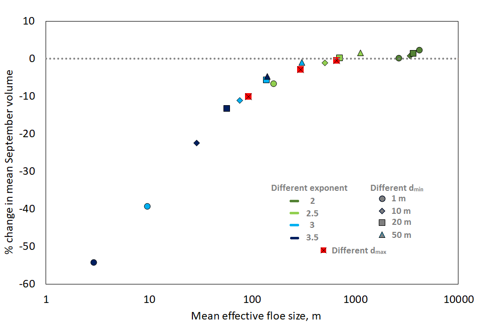
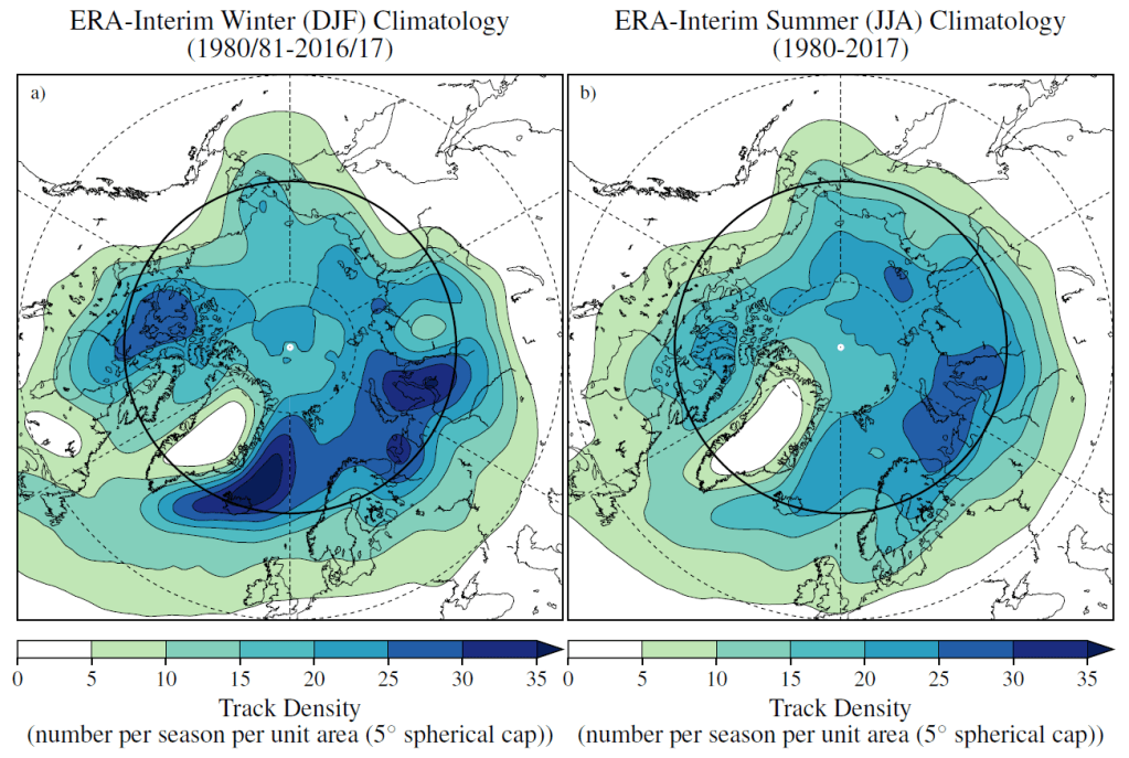
). Longitudes are shown every 60°E, and latitudes are shown at 80°N, 65°N (bold) and 50°N. Figure from Vessey at al. (2020).

In general, there is less consistency in Arctic storm characteristics in winter than in summer. This may be because in winter, the occurrence of meteorological conditions such as low level cloud, stable boundary layers and polar night that are more frequent, which are more challenging to represent in numerical weather prediction models, and for the creation of reanalysis datasets. In addition, there is a low density of conventional observations in winter, and difficulties in identifying cloud and estimating emissivity over snow and ice limit the current use of infrared and microwave satellite data in the troposphere (Jung et al. 2016).

The differences between the reanalysis datasets in Arctic storm frequency per season in winter (DJF) and summer (JJA) (1980-2017) were found to be less than 6 storms per season. On the other hand, the differences in Arctic storm frequency per season between storms identified by a storm tracking algorithm based on 850 hPa relative vorticity and MSLP were found to be 55 storms per season in winter, and 33 storms per season in summer. This shows that the decision to use 850 hPa relative vorticity or MSLP for storm tracking can be more important that the choice of reanalysis dataset.

Read more at: https://link.springer.com/article/10.1007/s00382-020-05142-4

References:

National Snow & Ice Data Centre (2019) Sea ice index. https://nsidc.org. Accessed 4 Mar 2019.

Reed RJ, Kunkel BA (1960) The Arctic circulation in summer. J. Meteorol. 17(5):489–506.

Sepp M, Jaagus J (2011) Changes in the activity and tracks of Arctic cyclones. Clim. Change 105(3–4):577–595.

Simmonds I, Burke C, Keay K (2008) Arctic climate change as manifest in cyclone behavior. J. Clim. 21(22):5777–5796.

Serreze MC, Barrett AP (2008) The summer cyclone maximum over the central Arctic Ocean. J. Clim. 21(5):1048–1065.

Vessey, A.F., Hodges, K.I., Shaffrey, L.C., Day, J.J., (2020) An inter‑comparison of Arctic synoptic scale storms between four global reanalysis datasets. Clim. Dyn., https://doi.org/10.1007/s00382-020-05142-4

Walsh, J.E., Bromwich, D.H., Overland, J.E., Serreze, M.C. and Wood, K.R., 2018. 100 years of progress in polar meteorology. Meteorological Monographs, 59, pp.21-1.

Zahn M, Akperov M, Rinke A, Feser F, Mokhov I I (2018) Trends of cyclone characteristics in the Arctic and their patterns from different reanalysis data. J. Geophys. Res. Atmos., 123(5):2737–2751.

The impact of atmospheric model resolution on the Arctic

Email: sally.woodhouse@pgr.reading.ac.uk

The Arctic region is rapidly changing, with surface temperatures warming at around twice the global average and sea ice extent is rapidly declining, particularly in the summer. These changes affect the local ecosystems and people as well as the rest of the global climate. The decline in sea ice has corresponded with cold winters over the Northern Hemisphere mid-latitudes and an increase in other extreme weather events (Cohen et al., 2014). There are many suggested mechanisms linking changes in the sea ice to changes in the stratospheric jet, midlatitude jet and storm tracks; however this is an area of active research, with much ongoing debate.

Stroeve_et_al-2012-fig2a
Figure 1. Time-series of September sea ice extent from 20 CMIP5 models (colored lines), individual ensemble members are dotted lines and the individual model mean is solid. Multi-model ensemble mean from a subset of the models is shown in solid black with +/- 1 standard deviation in dotted black. The red line shows observations. From Stroeve et al. (2012)

It is therefore important that we are able to understand and predict the changes in the Arctic, however there is still a lot of uncertainty. Stroeve et al. (2012) calculated time series of September sea ice extent for different CMIP5 models, shown in Figure 1. In general the models do a reasonable job of reproducing the recent trends in sea ice decline, although there is a large inter-model spread and and even larger spread in future projections. One area of model development is increasing the horizontal resolution – where the size of the grid cells used to calculate the model equations is reduced.

The aim of my PhD is to investigate the impact that climate model resolution has on the representation of the Arctic climate. This will help us understand the benefits that we can get from increasing model resolution. The first part of the project was investigating the impact of atmospheric resolution. We looked at three experiments (using HadGEM3-GC2), each at a different atmospheric resolutions: 135km (N512), 60km (N216) and 25km (N96).

sea_ice_concentration_obs_GC2
Figure 2. Annual mean sea ice concentration for observations (HadISST) and the bias of each different experiment from the observations N96: low resolution, N216: medium resolution, N512: high resolution.

The annual mean sea ice concentration for observations and the biases of the 3 experiments are shown in Figure 2. The low resolution experiment does a good job of producing the sea extent seen in observations with only small biases in the marginal sea ice regions. However, in the higher resolution experiments we find that the sea ice concentration is much lower than the observations, particularly in the Barents Sea (north of Norway). These changes in sea ice are consistent with warmer temperatures in the high resolution experiments compared to the low resolution.

To understand where these changes have come from we looked at the energy transported into the ocean by the atmosphere and the ocean. We found that there is an increase in the total energy being transported into the Arctic which is consistent with the reduced sea ice and warmer temperatures. Interestingly, the increase in energy is being transported into the Arctic by the ocean (Figure 3), even though it is the atmospheric resolution that is changing between the experiments. In the high resolution experiments the ocean energy transport into the Arctic, 0.15 petawatts (PW), is in better agreement with observational estimates, 0.154 PW, from Tsubouchi et al. (2018). Interestingly, this is in contrast to the worse representation of sea ice concentration in the high resolution experiments. (It is important to note that the model was tuned at the low resolution and as little as possible was changed when running the high resolution experiments which may contribute to the better sea ice concentration in the low resolution experiment.)

strait_locations
Location of ocean gateways into the Arctic. Red: Bering Strait, Green: Davis Strait, Blue: Fram Strait, Magenta: Barents Sea

ocean_heat_transport_GC2
Figure 3. Ocean energy transport for each resolution experiment through the four ocean gateways into the Arctic. The four gateways form a closed boundary into the Arctic.

We find that the ocean is very sensitive to the differences in the surface winds between the high and low resolution experiments. In different regions the differences in winds arise from different processes. In the Davis Strait the effect of coastal tiling is important, where at higher resolution a smaller area is covered by atmospheric grid cells that cover both land and ocean. In a cell covering both land and ocean the model usually produces wind speeds to low for over the ocean. Therefore in the higher resolution experiment we find that there are higher wind speeds over the ocean near the coast. Whereas over the Fram Strait and the Barents Sea instead we find that there are large scale atmospheric circulation changes that give the differences in surface winds between the experiments.

References

Cohen, J., Screen, J. A., Furtado, J. C., Barlow, M., Whittleston, D., Coumou, D., Francis, J., Dethloff, K., Entekhabi, D., Overland, J. & Jones, J. 2014: Recent Arctic amplification and extreme mid-latitude weather. Nature Geoscience, 7(9), 627–637, http://dx.doi.org/10.1038/ngeo2234

Stroeve, J. C., Kattsov, V., Barrett, A., Serreze, M., Pavlova, T., Holland, M., & Meier, W. N., 2012: Trends in Arctic sea ice extent from CMIP5, CMIP3 and observations. Geophysical Research Letters, 39(16), 1–7, https://doi.org/10.1029/2012GL052676

Tsubouchi, T., Bacon, S., Naveira Garabato, A. C., Aksenov, Y., Laxon, S. W., Fahrbach, E., Beszczynska-Möller, A., Hansen, E., Lee, C.M., Ingvaldsen, R. B. 2018: The Arctic Ocean Seasonal Cycles of Heat and Freshwater Fluxes: Observation-Based Inverse Estimates. Journal of Physical Oceanography, 48(9), 2029–2055, http://journals.ametsoc.org/doi/10.1175/JPO-D-17-0239.1

PhD Visiting Scientist 2019: Prof. Cecilia Bitz

r.frew@pgr.reading.ac.uk

With thanks to all my helpers who enabled the week to go smoothly! Adam Bateson, Sally Woodhouse, Kaja Milczewska and Agnieszka Walenkiewicz

Each year PhD students in the Department of Meteorology invite a distinguished scientist to spend a week with us.  This year we invited Prof. Cecilia Bitz, who visited between the 28th-31st May. Cecilia is based at the University of Washington, Seattle. 

Cecilia’s research interests are the role of sea ice in the climate system, and high latitude climate and climate change. She has also done a lot of work on the predictability of Arctic sea ice, and is involved in the Sea Ice Prediction Network.

The week began with a welcome reception in the coffee area, introducing Cecilia to the department, followed by a seminar by Cecilia on ‘Polar Regions as Sentinels of Different Climate Change’. The seminar predominantly focused on Antarctic sea ice, and the possible reasons why Antarctic sea ice behaviour is so different to the Arctic. Whilst Arctic sea ice has steadily declined we have seen Antarctic sea ice expansion over the past four decades, with extreme Antarctic sea ice extent lows since 2016.

Throughout the week Cecilia visited a number of the research groups, including Mesoscale, HHH (dynamics) and Cryosphere, where PhD students from each group presented to her, giving a taste of the range of PhD research within our department. 

Cecilia gave a second seminar later in the week in the Climate and Ocean Dynamics (COD) group meeting, this time focusing on the other pole, ‘Arctic Amplification: Local Versus Remote Causes and Consequences’. Cecilia discussed her work quantifying the role of feedbacks in Arctic Amplification, how they compare with meridional heat transports, and what influence Arctic warming has on the rest of the globe.

cuteness_on_ice
Photo Credit: Cecilia Bitz

On Wednesday afternoon the normal PhD group slot consisted of a career discussion, with Cecilia. Cecilia shared some of her career highlights with us, including extra opportunities she has taken such as doing some fieldwork in Antarctica and working for the charity, Polar Bears International, her insights and advice from her own experiences, as well as about post-doctoral opportunities in the US. A few of my personal take-aways from this session were to try give yourself space to learn one new thing at a time in your career (e.g. teaching, writing proposals, supervising etc). Try to work on a range of problems, and keep your outlook broad and open to new ideas and approaches. Take opportunities when they appear, such as fieldwork or short projects/collaborations. 

A small group of PhDs also met with her on the Friday to have an informal discussion about climate policy. In particular about her experiences speaking to the US senate, being a part of the IPCC reports and about the role of scientists in speaking about climate change, and whether we have a responsibility to do so.

Thursday evening the PhDs took Cecilia to Zero Degrees (a very apt choice for a polar researcher!), and enjoyed a lovely evening chatting over pizza and beer. 

The week ended with a farewell coffee morning on Friday, where we gave Cecilia some gifts to thank her for giving us her time this week including some tea, chocolates, a climate stripes mug and a framed picture of us… 

All the PhDs had a great week. We hope Cecilia enjoyed her visit as much as we did!

GroupPhoto
PhD students with Cecilia Bitz before the Careers Discussion.