Simon Lee, s.h.lee@pgr.reading.ac.uk
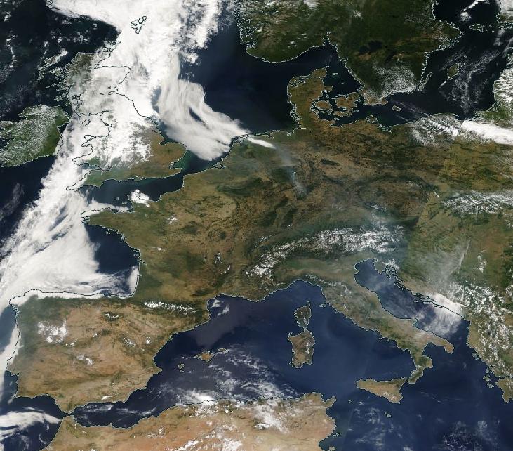
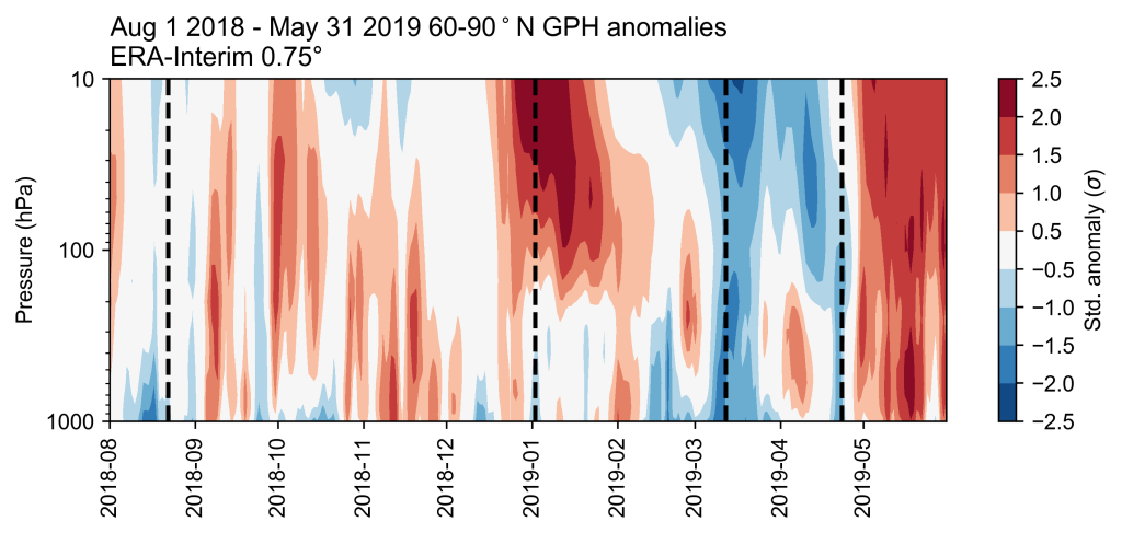
The February-March 2018 European cold-wave, known widely as “The Beast from the East” occurred around 2 weeks after a major sudden stratospheric warming (SSW) event on February 12th. Major SSWs typically occur once every other winter, involving significant disruption to the stratospheric polar vortex (a planetary-scale cyclone which resides over the pole in winter). SSWs are important because their occurrence can influence the type and predictability of surface weather on longer timescales of between 2 weeks to 2 months. This is known as subseasonal-to-seasonal (S2S) predictability, and “bridges the gap” between typical weather forecasts and seasonal forecasts (Figure 1).
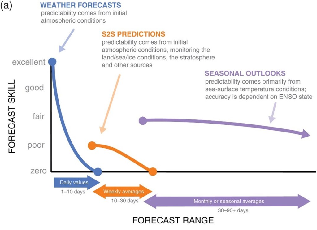
Figure 1: Schematic of medium-range, S2S and seasonal forecasts and their relative skill. [Figure 1 in White et al. (2017)]
In general, S2S forecasts suffer from relatively low skill. While medium-range forecasts are an initial value problem (depending largely on the initial conditions of the forecast) and seasonal forecasts are a boundary value problem (depending on slowly-varying constraints to the predictions, such as the El Niño-Southern Oscillation), S2S forecasts lie somewhere between the two. However, certain “windows of opportunity” can occur that have the potential to increase S2S skill – and a major SSW is one of them. Skilful S2S forecasts can be of particular benefit to public health planners, the transport sector, and energy demand management, among many others.
Following an SSW, the eddy-driven jet stream tends to weaken and shift equatorward. This is characteristic of the negative North Atlantic Oscillation (NAO) and negative Arctic Oscillation (AO), and during these patterns the risk of cold air outbreaks significantly increases in places like northwest Europe. So, by knowing this, S2S forecasts issued during the major SSW were able to highlight the increased risk of severely cold weather.
Given that we know that following an SSW certain weather types are more likely for several weeks, and forecasts may be more skilful, it might seem advantageous to know an SSW was coming at a long lead-time in order to really push the boundaries of S2S prediction. So, what about in 2018?
In the first paper from my PhD, published in July 2019 in JGR-Atmospheres, we explored the onset of predictions of the February 2018 SSW. We found that, until about 12 days beforehand, extended-range forecasts that contribute to the S2S database (an international collaboration of extended-range forecast data) did not accurately predict the event; in fact, most predictions indicated the vortex would remain unusually strong!
We diagnosed that anticyclonic wave breaking in the North Atlantic was a crucial synoptic-scale “trigger” event for perturbing the stratospheric vortex, by enhancing vertically propagating Rossby waves (which weaken the vortex when they break in the stratosphere). Forecasts struggled to predict this event far in advance, and thus struggled to predict the SSW. We called the pattern the “Scandinavia-Greenland (S-G) dipole” – characterised by an anticyclone over Scandinavia and a low over Greenland (Figure 2), and we found it was present before 35% of previous SSWs (1979-2018). The result agrees with several previous studies highlighting the role of blocking in the Scandinavia-Urals region, but was the first to suggest such a significant impact of a single tropospheric event.
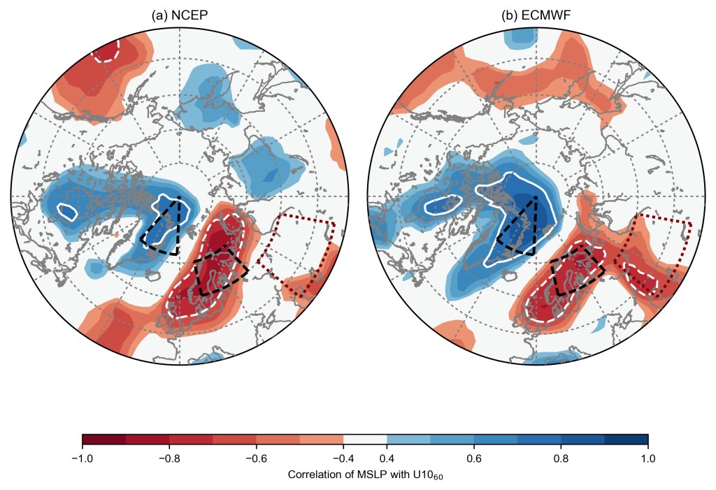
Figure 2: Correlation between mean sea level pressure forecasts over 3-5 February 2018 and subsequent forecasts of 10 hPa 60°N zonal-mean zonal wind on 9-11 February, in (a) NCEP and (b) ECMWF ensembles launched between 29 January and 1 February 2018. White lines (dashed negative) indicate correlations exceeding +/- 0.7, while the black dashed lines indicate the nodes of the S-G dipole. [Figure 3 in Lee et al. (2019)]
So, we had established the S-G dipole was important in the predictability onset in 2018, and important in previous cases – but how well do S2S models generally capture the pattern?
That was the subject of our recent (open-access) paper, published in August in QJRMS. We define a more generalised pattern by performing empirical orthogonal function (EOF) analysis on mean sea-level pressure anomalies in a region of the northeast Atlantic during November-March in ERA5 reanalysis (Figure 3). While the leading EOF (the “zonal pattern”) resembles the NAO, the 2nd EOF resembles the S-G dipole from our previous paper – so we call it the “S-G pattern”.
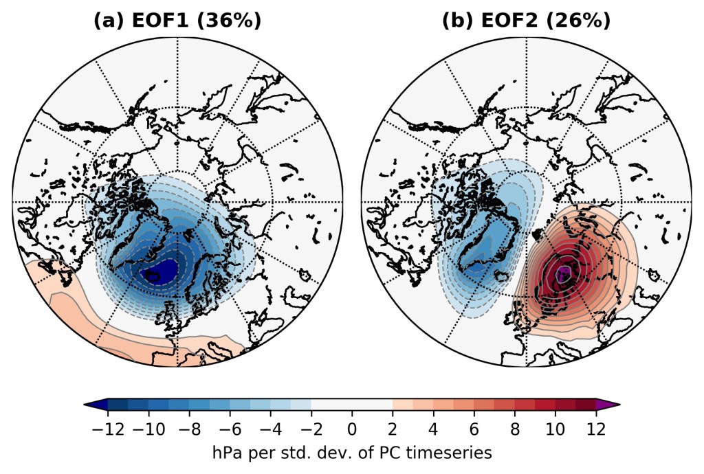
Figure 3: The first two leading EOFs of MSLP anomalies in the northeast Atlantic during November-March in ERA5, expressed as hPa per standard deviation of the principal component timeseries. The percentage of variance explained by the EOF is also shown. [Figure 1 in Lee et al. (2020)]
We then establish, through lagged linear regression analysis, that the S-G pattern is associated with enhanced vertically propagating wave activity (measured by zonal-mean eddy heat flux) into the stratosphere, and a subsequently weakened stratospheric vortex for the next 2 months. Thus, it supports our earlier work, and motivates considering how the pattern is represented in S2S models. To do this, we look at hindcasts – forecasts initialised for dates in the past – from 10 different prediction systems from around the world.
We find that while all the S2S models represent the spatial pattern of these two EOFs very well, some have biases in the variance explained by the EOFs, particularly at weeks 3 and 4 (Figure 4). Broadly, all the models have more variance explained by their first EOF compared with ERA5, and less by the second EOF – but this bias is particularly large for the three models with the lowest horizontal resolution (BoM, CMA, and HMCR).
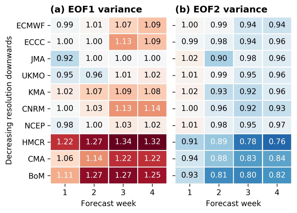
Figure 4: Weekly-mean ratio between the variance explained by the EOFs in each model and the ERA5 EOF. [Figure 6 in Lee et al. (2020)]
Additionally, we find that the deterministic prediction skill in the S-G pattern (measured by the ensemble-mean correlation) can be as small as 5-6 days for the BoM model – and only as high as 11 days in the higher resolution models. Extending this to probabilistic skill in weeks 3 and 4, we find models have only limited (if any) skill above climatology in weeks 3 and 4 (and much less than the skill in the leading EOF, the NAO-like pattern).
Furthermore, we find that the relationship between the S-G pattern and the enhanced heat flux in the stratosphere decays with lead-time in most S2S models, even in the higher-resolution models (Figure 5). Thus, this suggests that the dynamical link between the troposphere and stratosphere weakens with lead time in these models – so even a correct tropospheric prediction may not, in these cases, have a subsequently accurate extended-range stratospheric forecast.
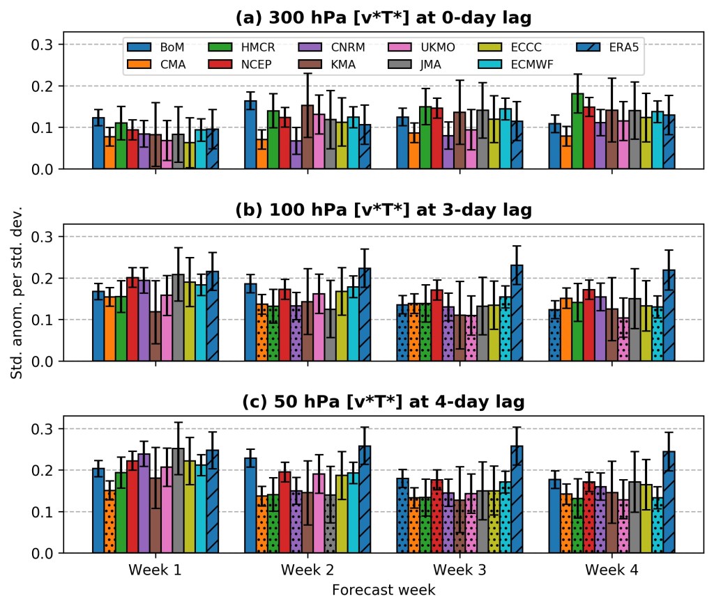
Figure 5: Weekly mean regression coefficients between the S–G index and the corresponding eddy heat flux anomalies at (a) 300 hPa on the same day, (b) 100 hPa three days later, and (c) 50 hPa four days later. The lags correspond to days with maximum correlation in ERA5. Stippled bars indicate a significant difference from ERA5 at the 95% confidence level. [Figure 11 in Lee et al. (2020)]
So, when taking this all together, we have:
- The S-G pattern is the second-leading mode of MSLP variability in the northeast Atlantic during winter.
- It is associated with enhanced vertically propagating wave activity into the stratosphere and a weakened polar vortex in the following weeks to months.
- S2S models represent the spatial patterns of the two leading EOFs well.
- Most S2S models have a zonal variability bias, with relatively more variance explained by the leading EOF and correspondingly less in the second EOF.
- This bias is largest in the lowest-resolution models in weeks 3 and 4.
- Extended range skill in the S-G pattern is low, and lower than for the NAO-like zonal pattern.
- The linear relationship between the S-G pattern and eddy heat flux in the stratosphere decays with lead-time in most S2S models.
The zonal variance bias is consistent with S2S model biases in Rossby wave breaking and blocking, while these biases have been widely found to be largest in the lowest resolution models. The results suggest that the poor prediction of the S-G event in February 2018 is not unique to that case, but a more generic issue. Overall, the combination of the variability biases, the poor extended-range predictability, and the poor representation of its impact on the stratospheric vortex at longer lead-times likely contributes to limiting skill at predicting major SSWs on S2S timescales – which remains low, despite the stratosphere’s much longer timescales. Correcting the biases outlined here will likely contribute to improving this skill, and subsequently increasing how far we are able to predict real-world weather.