Carl Haines – carl.haines@pgr.reading.ac.uk
In a recent blog post, I discussed the use of the analogue ensemble (AnEn), or “similar-day” approach to forecasting geomagnetic activity. In this post I will look at the use of support vector machines (SVMs), a machine learning approach, to the same problem and compare the performance of the SVM to the AnEn. An implementation of the SVM has been developed for this project in python and is available at https://doi.org/10.5281/zenodo.4604485.
Space weather encompasses a range of impacts on Earth caused by changes in the near-earth plasma due to variable activity at the Sun. These impacts include damage to satellites, interruptions to radio communications and damage to power grids. For this reason, it is useful to forecast the occurrence, intensity and duration of heightened geomagnetic activity, which we call geomagnetic storms.
As in the previous post, the measure of geomagnetic activity used is the aaH index which has been developed by Mike Lockwood in Reading. The aaH index gives a global measure of geomagnetic activity at a 3-hour resolution. In this index, the minimum value is zero and larger values represent more intense geomagnetic activity.
The SVM is a commonly used classification algorithm which we implement here to classify whether a storm will occur. Given a sample of the input and the associated classification labels, the SVM will find a function that separates these input features by their class label. This is simple if the classes are linearly separable, as the function is a hyperplane. The samples lying closest to the hyperplane are called support vectors and the distance between these samples and the hyperplane is maximised.
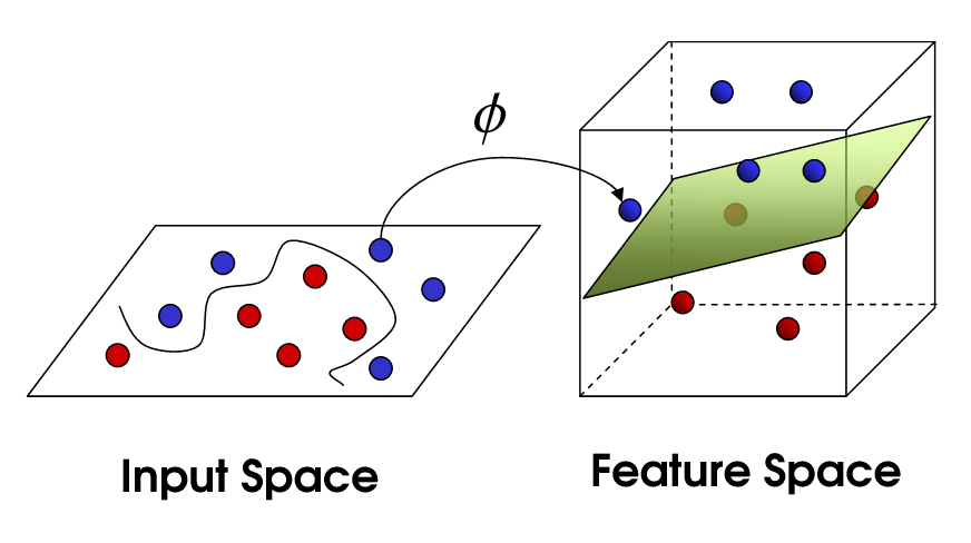
Typically, the samples are not linearly separable, so we employ Cover’s theorem which states that linearly inseparable classification problems are more likely to be linearly separable when cast non-linearly into a higher dimensional space. Therefore, we use a kenel trick to throw the inputs into a higher dimensional feature space, as depicted in Figure 1, to make it more separable. Further explanation is available in (Towards data science, n.d.)
Based on aaH values in the 24-hour training window, the SVM predicts whether the next 3 hours will be either a storm or not. By comparing this dichotomous hindcast with the observed aaH, the outcome will be one of True Positive (TP, where a storm is correctly predicted), True Negative (TN, where no storm is correctly predicted), False Positive (FP, where a storm is predicted but not observed), or False Negative (FN, where a storm is not predicted but is observed). This is shown in the form of a contingency table in Figure 2.

For development of the SVM, the aaH data has been separated into independent training and test intervals. These intervals are chosen to be alternate years. This is longer than the auto-correlation in the data (choosing, e.g. alternate 3-hourly data points, would not generate independent training and test data sets) but short enough that we assume there will not be significant aliasing with solar cycle variations.
Training is an iterative process, whereby a cost function is minimised. The cost function is a combination of the relative proportion of TP, TN, FP and FN. Thus, while training itself, an SVM attempts to classify labelled data i.e., data belonging to a known category, in this case “storm” and “no storm” on the basis of the previous 24 hours of aaH. If the SVM makes an incorrect prediction it is penalised through a cost function which the SVM minimises. The cost parameter determines the degree to which the SVM is penalised for a misclassification in training which allows for noise in the data.
It is common that data with a class imbalance, that is containing many more samples from one class than the other, causes the classifier to be biased towards the majority class. In this case, there are far more non-storm intervals than storm intervals. Following (McGranaghan, Mannucci, Wilson, Mattman, & Chadwick, 2018), we define the cost of mis-classifying each class separately. This is done through the weight ratio Wstorm : Wno storm. Increasing the Wstorm increases the frequency at which the SVM predicts a storm and it follows that it predicts no storm at a reduced frequency. In this work we have varied Wstorm and kept Wno storm constant at 1. A user of the SVM method for forecasting may wish to tune the class weight ratio to give an appropriate ratio of false alarms and hit rate dependent on their needs.
Different forecast applications will have different tolerances for false alarms and missed events. To accommodate this, and as a further comparison of the hindcasts, we use a Cost/Loss analysis. In short, C is the economic cost associated with taking mitigating action when an event is predicted (whether or not it actually occurs) and L is the economic loss suffered due to damage if no mitigating action is taken when needed. For a deterministic method, such as the SVM, each time a storm is predicted will incur a cost C. Each time a storm is not predicted but a storm occurs a loss L is incurred. If no storm is predicted and no storm occurs, then no expense in incurred. By considering some time interval, the total expense can be computed by summing C and L. Further information, including the formular for computing the potential economic value (PEV) can be found in (Owens & Riley, 2017).
A particular forecast application will have a C/L ratio in the domain (0,1). This is because a C/L of 0 would mean it is most cost effective to take constant mitigating action and a C/L of 1 or more means that mitigating action is never cost effective. In either case, no forecast would be helpful. The power of a Cost/Loss analysis is that it allows us to evaluate our methods for the entire range of potential forecast end users without specific knowledge of the forecast application requirements. End users can then easily interpret whether our methods fit their situation.
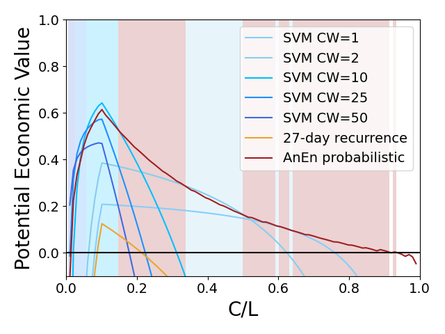
Figure 3 shows the potential economic value (PEV) of the SVM with a range of class weights (CW), probabilistic AnEn and 27-day recurrence. The shaded regions indicate which hindcast has the highest PEV for that Cost/Loss ratio. The probabilistic AnEn has the highest PEV for the majority of the Cost/Loss domain although SVM has higher PEV for lower Cost/Loss ratios. It highlights that the `best’ hindcast is dependent on the context in which it is to be employed.
In summary, we have implemented an SVM for the classification of geomagnetic storms and compared the performance to that of the AnEn which was discussed in a previous blog post. The SVM and AnEn generally perform similarly in a Cost/Loss analysis and the best method will depend on the requirements of the end user. The code for the SVM is available at https://doi.org/10.5281/zenodo.4604485 and the AnEn at https://doi.org/10.5281/zenodo.4604487.
References
Burges, C. (1998). A tutorial on support vector machines for pattern recognition. Data mining an knowledge discovery.
McGranaghan, R., Mannucci, A., Wilson, B., Mattman, C., & Chadwick, R. (2018). New Capabilities for Prediction of High-Latitude Ionospheric Scin-669tillation: A Novel Approach With Machine Learning. Space Weather.
Owens, M., & Riley, P. (2017). Probabilistic Solar Wind Forecasting Using Large Ensembles of Near-Sun Conditions With a Simple One-Dimensional “Upwind” Scheme. Space weather.
Towards data science. (n.d.). Retrieved from https://towardsdatascience.com/the-kernel-trick-c98cdbcaeb3f
