Understanding the dynamics of cyclone clustering

Priestley, M. D. K., J. G. Pinto, H. F. Dacre, and L. C. Shaffrey (2016), Rossby wave breaking, the upper level jet, and serial clustering of extratropical cyclones in western Europe, Geophys. Res. Lett., 43, doi:10.1002/2016GL071277.

Email: m.d.k.priestley@pgr.reading.ac.uk

Extratropical cyclones are the number one natural hazard that affects western Europe (Della-Marta, 2010). These cyclones can cause widespread socio-economic damage through extreme wind gusts that can damage property, and also through intense precipitation, which may result in prolonged flood events. For example the intensely stormy winter of 2013/2014 saw 456mm of rain fall in under 90 days across the UK; this broke records nationwide as 175% of the seasonal average fell (Kendon & McCarthy, 2015). One particular storm in this season was cyclone Tini (figure 1), this was a very deep cyclone (minimum pressure – 952 hPa) which brought peak gusts of over 100 mph to the UK. These gusts caused widespread structural damage that resulted in 20,000 homes losing power. These extremes can be considerably worse when multiple extratropical cyclones affect one specific geographical region in a very short space of time. This is known as cyclone clustering. Some of the most damaging clustering events can result in huge insured losses, for example the storms in the winter of 1999/2000 resulted in €16 billion of losses (Swiss Re, 2016); this being more than 10 times the annual average.

figure-1
Figure 1. A Meteosat visible satellite image at 12 UTC on February 12th 2014 showing cyclone Tini over the UK. Image credit to NEODAAS/University of Dundee.

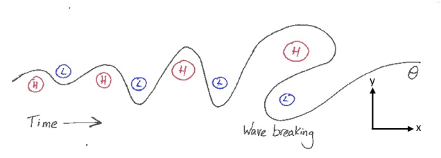
Up until recently cyclone clustering had been given little attention in terms of scientific research, despite it being a widely accepted phenomenon in the scientific community. With these events being such high risk events it is important to understand the atmospheric dynamics that are associated with these events; and this is exactly what we have been doing recently. In our new study we attempt to characterise cyclone clustering in several different locations and associate each different set of clusters with a different dynamical setup in the upper troposphere. The different locations we focus on are defined by three areas, one encompassing the UK and centred at 55°N. Our other two areas are 10° to the north and south of this (centred at 65°N and 45°N.) The previous study of Pinto et al. (2014) examined several winter seasons and found links between the upper-level jet, Rossby wave breaking (RWB) and the occurrence of clustering. RWB is the meridional overturning of air in the upper troposphere. It is identified using the potential temperature (θ) field on the dynamical tropopause, with a reversal of the normal equator-pole θ gradient representing RWB. This identification method is explained in full in Masato et al. (2013) and also illustrated in figure 2. We have greatly expanded on this analysis to look at all winter clustering events from 1979/1980 to 2014/2015 and their connection with these dynamical features.

schematic_box1
Figure 2. Evolution of Rossby waves on the tropopause. RWB occurs when these waves overturn by a significant amount. H: High potential temperature; L: Low potential temperature (Priestley et al., 2017).

We find that when we get clustering it is accompanied with a much stronger jet at 250 hPa than in the climatology, with average speeds peaking at over 50 ms-1 (figures 3a-c). In all cases there is also a much greater presence of RWB in regions not seen from the climatology (Figure 3d). In figure 3a there is more RWB to the south of the jet, in figure 3b there is an increased presence on both the northern and southern flanks, and finally in figure 3c there is much more RWB to the north. The presence of this anomalous RWB transfers momentum into the jet, which acts to strengthen and extend it toward western Europe.

figure-2
Figure 3. The dynamical setup for clustering occurring at (a) 65°N; (b) 55°N; and (c) 45°N. The climatology is shown in (d). Coloured shading is the average potential temperature on the tropopause, black contours are the average 250 hPa wind speeds and black crosses are where RWB is occurring.

The location of the RWB controls the jet tilt; more RWB to the south of the jet acts to angle it more northwards (figure 3a), there is a southward deflection when there is more RWB to the north of the jet (figure 3c). The presence of RWB on both sides extends it along a more central axis (figure 3b). Therefore the occurrence of RWB in a particular location and the resultant angle of the jet acts to direct cyclones to various parts of western Europe in quick succession.

In our recently published study we go into much more detail regarding the variability associated with these dynamics and also how the jet and RWB interact in time. This can be found at http://dx.doi.org/10.1002/2016GL071277.

This work is funded by NERC via the SCENARIO DTP and is also co-sponsored by Aon Benfield.

References

Della-Marta, P. M., Liniger, M. A., Appenzeller, C., Bresch, D. N., Köllner-Heck, P., & Muccione, V. (2010). Improved estimates of the European winter windstorm climate and the risk of reinsurance loss using climate model data. Journal of Applied Meteorolo

Kendon, M., & McCarthy, M. (2015). The UK’s wet and stormy winter of 2013/2014. Weather, 70(2), 40-47.

Masato, G., Hoskins, B. J., & Woollings, T. (2013). Wave-breaking characteristics of Northern Hemisphere winter blocking: A two-dimensional approach. Journal of Climate, 26(13), 4535-4549.

Pinto, J. G., Gómara, I., Masato, G., Dacre, H. F., Woollings, T., & Caballero, R. (2014). Large‐scale dynamics associated with clustering of extratropical cyclones affecting Western Europe. Journal of Geophysical Research: Atmospheres, 119(24).

Priestley, M. D. K., J. G. Pinto, H. F. Dacre, and L. C. Shaffrey (2017). The role of cyclone clustering during the stormy winter of 2013/2014. Manuscript in preparation.

Swiss Re. (2016). Winter storm clusters in Europe, Swiss Re publishing, Zurich, 16 pp., http://www.swissre.com/library/winter_storm_clusters_in_europe.html. Accessed 24/11/16.

Geoengineering – how could we detect its cooling effect?

Detecting sulphate aerosol geoengineering with different methods
Lo, Y. T. E. et al. Detecting sulphate aerosol geoengineering with different methods. Sci. Rep. 6, 39169; doi: 10.1038/srep39169 (2016).

Email: y.t.e.lo@pgr.reading.ac.uk

Sulphate aerosol injection (SAI) is one of the geoengineering proposals that aim to reduce future surface temperature rise in case ambitious carbon dioxide mitigation targets cannot be met.  Climate model simulations suggest that by injecting 5 teragrams (Tg) of sulphur dioxide gas (SO2) into the stratosphere every year, global surface cooling would be observed within a few years of implementation.  This injection rate is equivalent to 5 million tonnes of SOper year, or one Mount Pinatubo eruption every 4 years (large volcanic eruptions naturally inject SOinto the stratosphere; the Mount Pinatubo eruption in 1991 led to ~0.5 °C global surface cooling in the 2 years that followed (Self et al., 1993)).  However, temperature fluctuations occur naturally in the climate system too.  How could we detect the cooling signal of SAI amidst internal climate variability and temperature changes driven by other external forcings?

The answer to this is optimal fingerprinting (Allen and Stott, 2003), a technique which has been extensively used to detect and attribute climate warming to human activities.  Assuming a scenario (G4, Kravitz et al., 2011) in which 5 Tg yr-1 of SO2 is injected into the stratosphere on top of a mid-range warming scenario called RCP4.5 from 2020-2070, we first estimate the climate system’s internal variability and the temperature ‘fingerprints’ of the geoengineering aerosols and greenhouse gases separately, and then compare observations to these fingerprints using total least squares regression.  Since there are no real-world observations of geoengineering, we cross-compare simulations from different climate models in this research.  This gives us 44 comparisons in total, and the number of years that would be needed to robustly detect the cooling signal of SAI in global-mean near-surface air temperature is estimated for each of them.

Figure 1(a) shows the distribution of the estimated time horizon over which the SAI cooling signal would be detected at the 10% significance level in these 44 comparisons.  In 29 of them, the cooling signal would be detected during the first 10 years of SAI implementation.  This means we would not only be able to separate the cooling effect of SAI from the climate system’s internal variability and temperature changes driven by greenhouse gases, but we would also be able to achieve this early into SAI deployment.

eunice_blog_1_fig1
Figure 1: Distribution of the estimated detection horizons of the SAI fingerprint using (a) the conventional two-fingerprint detection method and (b) the new, non-stationary detection method.

The above results are tested by applying a variant of optimal fingerprinting to the same problem.  This new method assumes a non-stationary background climate that is mainly forced by greenhouse gases, and attempts to detect the cooling effect of SAI against the warming background using regression (Bürger and Cubasch, 2015).  Figure 1(b) shows the distribution of the detection horizons estimated by using the new method in the same 44 comparisons: 35 comparisons would require 10 years or fewer for the cooling signal to be robustly detected.  This shows a slight improvement from the results found with the conventional method, but the two distributions are very similar.

To conclude, we would be able to separate and thus, detect the cooling signal of sulphate aerosol geoengineering from internal climate variability and greenhouse gas driven warming in global-mean temperature within 10 years of SAI deployment in a future 5 Tg yr-1 SAI scenario.  This could be achieved with either the conventional optimal fingerprinting method or a new, non-stationary detection method, provided that the climate data are adequately filtered.  Research on the effects of different data filtering techniques on geoengineering detectability is not included in this blog post, please refer to the article cited at the top for more details.

This work has been funded by the University of Reading.  Support has also been provided by the UK Met Office.

Note: So how feasible is a 5 Tg yr-1 SO2 injection scenario?  Robock et al. (2009) estimated the cost of lofting 1 Tg yr-1 SO2 into the stratosphere with existing aircrafts to be several billion U.S. dollars per year. Scaling this to 5 Tg yr-1 is still not a lot compared to the gross world product. There are practical issues to be addressed even if existing aircrafts were to be used for SAI, but the deciding factor of whether to implement sulphate aerosol geoengineering or not would likely be its potential benefits and side effects, both on the climate system and the society. 


References

Self, Stephen, et al. “The atmospheric impact of the 1991 Mount Pinatubo eruption.” (1993).

Allen, M. R., and P. A. Stott. “Estimating signal amplitudes in optimal fingerprinting, Part I: Theory.” Climate Dynamics 21.5-6 (2003): 477-491.

Kravitz, Ben, et al. “The geoengineering model intercomparison project (GeoMIP).” Atmospheric Science Letters 12.2 (2011): 162-167.

Bürger, Gerd, and Ulrich Cubasch. “The detectability of climate engineering.” Journal of Geophysical Research: Atmospheres 120.22 (2015).

Robock, Alan, et al. “Benefits, risks, and costs of stratospheric geoengineering.” Geophysical Research Letters 36.19 (2009).

AGU Fall Meeting – Posters and Protests

Email: r.e.emerton@pgr.reading.ac.uk

From 12th to 16th December 2016, the annual American Geophysical Union (AGU) Fall Meeting took place at the Moscone Centre in San Francisco. AGU remains the largest Earth and Space Science conference in the world with more than 25,000 scientists.

agu
Overlooking the Poster Hall in Moscone South

At the 2016 Fall Meeting, I was one of around 8000 students who arrived in San Francisco to present one of the 15,000 posters that would be displayed over the course of the week. While I knew that AGU is one of the largest Earth science conferences, and had indeed spent hours on the plane fine-tuning my schedule to choose which of the ~200 hydrology sessions (let alone the meteorology sessions also related to my work) I would attend, the scope and diversity of the research presented throughout the week really sunk in when I stood on the mezzanine overlooking the poster hall on the first day of the conference.

I was lucky enough to be awarded an AGU student travel grant in order to present my latest PhD research that I’ve been working on at the University of Reading, in collaboration with the European Centre for Medium-Range Weather Forecasts (ECMWF), and funded by NERC as part of the SCENARIO Doctoral Training Partnership. My work maps the historical probability of increased (or decreased) flood hazard across the globe during ENSO (El Niño and La Niña) events, using the first 20th Century ensemble river flow reanalysis, created at ECMWF as part of this work. But more on that another time!

blogpostscreenshotUnlike other conferences I’d presented at, the poster sessions at AGU span half a day – while you are only expected to be there to discuss the work for two hours, it’s inevitable that you get caught up in discussion and I saw many presenters (myself included) who stuck by their poster for the full 4.5 hours! I thoroughly enjoyed my poster session, where several familiar faces dropped by for an update on my work, and others stopped to pose new questions and make a few suggestions for improvements to my maps (wait, why didn’t I think of that?!). As a student presenter, I could also register for the Outstanding Student Poster Award – which means that my poster was anonymously judged, and I will soon be receiving  feedback on my poster and presentation – an opportunity I was excited about to make sure I continue to improve the way I communicate my research.

For me, some of the sessions that were highlights of the conference included  ‘Global Floods: Forecasting, Monitoring, Risk Assessment and Socioeconomic Response‘, ‘Large-scale Climate Variability and its Impact on Hydrological Systems, Water Resources and Population‘, ‘Forecasting Hydrology at Continental Scale‘, ‘Transforming Hydrologic Prediction and Decision Making: Uncertainty’ and ‘ENSO Dynamics, Observations and Predictability in light of the 2015-2016 El Niño Event‘. With such a range of science being presented, there’s also plenty of opportunity (well, so long as you haven’t double- or triple-booked sessions in your schedule already!) to listen to talks outside of your own field – which is how I ended up in an 8am talk on operational earthquake forecasting and early warning. It was brilliant to learn about forecasting natural hazards outside of hydrology and meteorology!

There was also the social aspect that’s a big part of any conference – networking, networking and more networking! While it can be daunting, particularly at a conference of this size, to find and introduce yourself to scientists in your field whose work you’ve read but you’ve never met, I was pleased to first bump into some friendly faces who in turn introduced me to the new faces. Plus, it’s an AGU tradition that ‘AGU beer’ is served at 3.30pm sharp and the conference centre fills with groups of friends and colleagues in heated debates and discussions about anything from volcanoes to Jupiter’s magnetosphere.

It was impossible not to notice, however, the many more politically-themed conversations than would normally be overheard at such an event, as a result of uncertainty about the future of science in light of the recent US presidential election. While I was in the middle of research discussions at my poster, a ‘Stand up for Science‘ rally took place a few blocks away from the conference centre, where scientists donned lab coats and held signs – “stand up for science”, “ice has no agenda – it just melts” – protesting to raise awareness of the challenges, and to support science. You can read the Guardian article here.

blogscreenshot2

All in all, AGU was a brilliant chance to present and discuss part of my research that I had just finished – it was certainly overwhelming and tough to choose which sessions to stop by (which meant I missed one or two presentations that sounded great), but I would recommend it for showcasing your work (and receiving feedback via the OSPA) and meeting scientists in your field that you wouldn’t normally bump into at conferences in Europe, especially if you can apply for one of AGU’s travel grants to help cover the costs of getting there.

P.S. You can watch presentations from the AGU Fall Meeting 2016 on the website.

Of course, I couldn’t fly all the way out to California and not find time to explore San Francisco a little.


From foehn to intense rainfall: the importance of Alps in influencing the regional weather

Email: a.volonte@pgr.reading.ac.uk

dsc_0196
Figure 1: View from Monte Lema (Italy-Switzerland) looking West. The Lake Maggiore region and the southern Alpine foothills are visible in the foreground whereas Monte Rosa and the Pennine Alps behind them are partially hidden by a characteristic foehn wall.  (A. Volonté, 4 January 2017)

The interaction between atmospheric flow and topography is at the origin of various important weather phenomena, as we have already seen in Carly Wright’s blog post. When a mountain range is particularly high and extended it can even block or deflect weather systems, as it happens with the Alps. For example, in Figure 1 we can see the main Alpine range with its over-4000m-high peaks blocking a cold front coming from the north. The main ridge acts as a wall, enhancing condensation and precipitation processes on the upstream side (stau condition) and leaving clear skies on the downstream lee side, where dry and mild katabatic foehn winds flow. The contrast is striking between sunny weather on Lake Maggiore and snowy conditions over Monte Rosa, just a few miles apart. The same phenomenon is shown in Figure 2 with a satellite image that highlights how a cold front coming from northwest gets blocked by the Alpine barrier. A person enjoying the sunny day in the southern side of the Alps, if unaware of this mechanism, would be very surprised  to know that the current weather is so different on the other side of the range.

poplex-2014295-terra-1km
Figure 2: Satellite image (MODIS-NASA) over the Alps and Po Valley on 22 October 2014
poplex-2016348-terra-1km
Figure 3: same as Figure 1 but on 13 December 2016

A comparison with Figure 3 helps to notice that in Figure 2 the shape of the cloud band closely mirrors the mountain range. As an additional remark,  this comparison shows that foehn bring clear skies even in the Po Valley, having blown away the typical mist/fog occurring in the region in Autumn and Winter months in high pressure regimes. The  stau/foehn dynamics is actually very fascinating, and you can read more about it in Elvidge and Renfrew (2015 ) and in Miltenberger et al. (2016), among others. Unfortunately, the interaction of weather systems with the Alps can often trigger very damaging phenomena, like heavy and long-lasting precipitation on one side of the slope, and this is what the rest of this post will be focused on. In fact, the most recent event of this kind just happened at the end of November, with intense and long-lasting rain affecting the southern slope of the Alps  and causing floods particularly in the Piedmont region, in northwestern Italy ( Figure 4).

tanaro2
Figure 4: River Tanaro flooding in the town of Garessio, 24 November 2016 (Piedmont, Italy). Source: http://www.corrierenazionale.it
arpa_piemonte
Figure 5: rainfall accumulated between 21 and 26 November 2016 in the Piedmont region. Source: Regional Agency for the protection of the Environment – Piedmont

Figure 5 shows that the accumulated rainfall in the event goes over 300 mm in a large band that follows the shape of the southern Alpine slope in the region (see map of Piedmont, from Google Maps), reaching even 600 mm in a few places. This situation is the result of moist southerly flow being blocked by the Alps and thus causing ascent and consequent precipitation to persist on the same areas for up to five days. It is quite common to see quasi-stationary troughs enter the Mediterranean region during Autumn months causing strong and long-lasting moist flows to move towards the Alps. Hence, it is crucial to understand  where the heaviest precipitation will occur. In other words, will it rain the most on top of the ridge or on the upstream plain? What processes are controlling the location of heavy precipitation with respect to the slope?

The study published by Davolio et al. (2016), available here and originated from my master degree’s thesis, tackles this issue focusing on northeastern Italy. In fact, the analysis includes three case studies in which heavy and long-lasting rain affected the eastern Alps and other three case studies in which intense rainfall was mainly located on the upstream plain. Although all the events showed common large-scale patterns and similar mesoscale settings, characterised by moist southerly low-level flow interacting with the Alps, the rainfall distribution turned out to be very dissimilar. The study highlights that the two precipitation regimes strongly differ in terms of interaction of the flow with the mountain barrier. When the flow is able to go over the Alps the heaviest rain occurs on top of the ridge. When the flow is instead blocked and deflected by the ridge (flow around), creating a so-called barrier wind, intense convection is triggered on the upstream plain (Figure 6) .

qj2731
Figure 6: Schematic diagram of the key mechanisms governing the two different wind and precipitation patterns over NE Italy. (a) Blocked low-level flow, barrier wind, convergence and deep convection over the plain, upstream the orography. (b) Flow over conditions with orographic lifting and precipitation mainly over the Alps. From Davolio et al. (2016)
convection
Figure 7: cross section going from the Adriatic Sea to the Alps in one of the events simulated. Equivalent potential temperature is shaded, thick black lines indicate clouds while arrows show tangent wind component. See Davolio et al. (2016)

The key mechanism that explains this different evolution is connected to the thermodynamic state of the impinging flow. In fact, when the southerly moist and warm air gets close to the Alpine barrier it is lifted above the colder air already present at the base of the orography. It can be said that the colder air behaves as a first effective mountain for the incoming flow. If this lifting process triggers convection, then the persistence of a blocked-flow condition is highly favoured (see Figure 7). On the contrary, if this initial lifting process does not trigger convection the intense moist flow will eventually be able to go over the ridge, where a more substantial ascent will take place, causing heavy rain on the ridge top. This study also looks at numerical parameters used in more idealised analyses (like in Miglietta and Rotunno (2009)), finding a good agreement with the theory.

To summarise, we can say that the Alpine range is able to significantly modify weather systems when interacting with them. Thus, an in-depth understanding of the processes taking place during the interaction, along with a coherent model is necessary to capture correctly the effects on the local weather, being either a rainfall enhancement, the occurrence of foehn winds or various other phenomena.

References

Davolio, S., Volonté A., Manzato A., Pucillo A., Cicogna A. and Ferrario M.E. (2016), Mechanisms producing different precipitation patterns over north-eastern Italy: insights from HyMeX-SOP1 and previous events. Q.J.R. Meteorol. Soc., 142 (Suppl 1): 188-205. doi:10.1002/qj.2731

Elvidge A. D., Renfrew, I. A. (2015). The causes of foehn warming in the lee of mountains. Bull. Am. Meteorol. Soc. 97: 455466, doi:10.1175/BAMS-D-14-00194.1.

Miglietta M. and Rotunno R., (2009) Numerical Simulations of Conditionally Unstable Flows over a Mountain Ridge. J. Atmos. Sci., 66, 1865–1885, doi: 10.1175/2009JAS2902.1. 

Miltenberger, A. K., Reynolds, S. and Sprenger, M. (2016), Revisiting the latent heating contribution to foehn warming: Lagrangian analysis of two foehn events over the Swiss Alps. Q.J.R. Meteorol. Soc., 142: 2194–2204. doi:10.1002/qj.2816