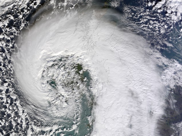
Figure 1: Windstorm Tini (12 Feb 2014) passes over the British Isles bringing extreme winds. A Sting Jet has been identified in the storm. Image courtesy of NASA Earth Observatory
It was the morning of 16th October when South East England got battered by the Great Storm of 1987. Extreme winds occurred, with gusts of 70 knots or more recorded continually for three or four consecutive hours and maximum gusts up to 100 knots. The damage was huge across the country with 15 million trees blown down and 18 fatalities.
Figure 2: Surface wind gusts in the Great Storm of 1987. Image courtesy of UK Met Office.
The forecast issued on the evening of 15th October failed to identify the incoming hazard but forecasters were not to blame as the strongest winds were actually due to a phenomenon that had yet to be discovered at the time: the Sting Jet. A new topic of weather-related research had started: what was the cause of the exceptionally strong winds in the Great Storm?
It was in Reading at the beginning of 21st century that scientists came up with the first formal description of those winds, using observations and model simulations. Following the intuitions of Norwegian forecasters they used the term Sting Jet, the ‘sting at the end of the tail’. Using some imagination we can see the resemblance of the bent-back cloud head with a scorpion’s tail: strong winds coming out from its tip and descending towards the surface can then be seen as the poisonous sting at the end of the tail.
Figure 3: Conceptual model of a sting-jet extratropical cyclone, from Clark et al, 2005. As the cloud head bends back and the cold front moves ahead we can see the Sting Jet exiting from the cloud tip and descending into the opening frontal fracture. WJ: Warm conveyor belt. CJ: Cold conveyor belt. SJ: Sting jet.
In the last decade sting-jet research progressed steadily with observational, modelling and climatological studies confirming that the strong winds can occur relatively often, that they form in intense extratropical cyclones with a particular shape and are caused by an additional airstream that is neither related to the Cold nor to the Warm Conveyor Belt. The key questions are currently focused on the dynamics of Sting Jets: how do they form and accelerate?
Works recently published (and others about to come out, stay tuned!) claim that although the Sting Jet occurs in an area in which fairly strong winds would already be expected given the morphology of the storm, a further mechanism of acceleration is needed to take into account its full strength. In fact, it is the onset of mesoscale instabilities and the occurrence of evaporative cooling on the airstream that enhances its descent and acceleration, generating a focused intense jet (see references for more details). It is thus necessary a synergy between the general dynamics of the storm and the local processes in the cloud head in order to produce what we call the Sting Jet .
Figure 4: Sting Jet (green) and Cold Conveyor Belt (blue) in the simulations of Windstorm Tini. The animation shows how the onset of the strongest winds is related to the descent of the Sting Jet. For further details on this animation and on the analysis of Windstorm Tini see here.
Browning, K. A. (2004), The sting at the end of the tail: Damaging winds associated with extratropical cyclones. Q.J.R. Meteorol. Soc., 130: 375–399. doi:10.1256/qj.02.143
Clark, P. A., K. A. Browning, and C. Wang (2005), The sting at the end of the tail: Model diagnostics of fine-scale three-dimensional structure of the cloud head. Q.J.R. Meteorol. Soc., 131: 2263–2292. doi:10.1256/qj.04.36
Martínez-Alvarado, O., L.H. Baker, S.L. Gray, J. Methven, and R.S. Plant (2014), Distinguishing the Cold Conveyor Belt and Sting Jet Airstreams in an Intense Extratropical Cyclone. Mon. Wea. Rev., 142, 2571–2595, doi: 10.1175/MWR-D-13-00348.1.
Hart, N.G., S.L. Gray, and P.A. Clark, 0: Sting-jet windstorms over the North Atlantic: Climatology and contribution to extreme wind risk. J. Climate, 0, doi: 10.1175/JCLI-D-16-0791.1.
Volonté, A., P.A. Clark, S.L. Gray. The role of Mesoscale Instabilities in the Sting-Jet dynamics in Windstorm Tini. Poster presented at European Geosciences Union – General Assembly 2017, Dynamical Meteorology (General session)
Gristey, J. J., J. C. Chiu, R. J. Gurney, S.-C. Han, and C. J. Morcrette (2017), Determination of global Earth outgoing radiation at high temporal resolution using a theoretical constellation of satellites, J. Geophys. Res. Atmos., 122, doi:10.1002/2016JD025514.
The surface of our planet has warmed at an unprecedented rate since the mid-19th century and there is no sign that the rate of warming is slowing down. The last three decades have all been successively warmer than any preceding decade since 1850, and 16 of the 17 warmest years on record have all occurred since 2001. The latest science now tells us that it is extremely likely that human influence has been the dominant cause of the observed warming1, mainly due to the release of carbon dioxide and other greenhouse gases into our atmosphere. These greenhouse gases trap heat energy that would otherwise escape to space, which disrupts the balance of energy flows at the top of the atmosphere (Fig. 1). The current value of the resulting energy imbalance is approximately 0.6 W m–2, which is more than 17 times larger than all of the energy consumed by humans2! In fact, observing the changes in these energy flows at the top of the atmosphere can help us to gauge how much the Earth is likely to warm in the future and, perhaps more importantly, observations with sufficient spatial coverage, frequency and accuracy can help us to understand the processes that are causing this warming.
Figure 1. The Earth’s top-of-atmosphere energy budget. In equilibrium, the incoming sunlight is balanced by the reflected sunlight and emitted heat energy. Greenhouse gases can reduce the emitted heat energy by trapping heat in the Earth system leading to an energy imbalance at the top of the atmosphere.
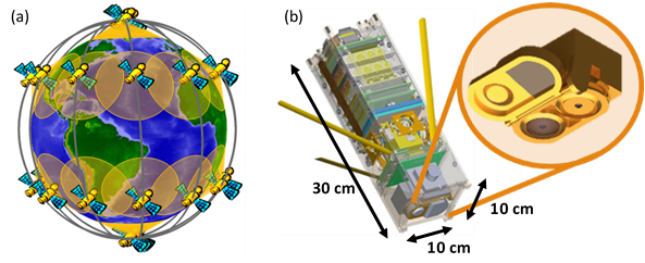
Observations of energy flows at the top of the atmosphere have traditionally been made by large and expensive satellites that may be similar in size to a large car3, making it impractical to launch multiple satellites at once. Although such observations have led to many advancements in climate science, the fundamental sampling restrictions from a limited number of satellites makes it impossible to fully resolve the variability in the energy flows at the top of atmosphere. Only recently, due to advancements in small satellite technology and sensor miniaturisation, has a novel, viable and sustainable sampling strategy from a constellation of satellites become possible. Importantly, a constellation of small satellites (Fig. 2a), each the size of a shoe-box (Fig. 2b), could provide both the spatial coverage and frequency of sampling to properly resolve the top of atmosphere energy flows for the first time. Despite the promise of the constellation approach, its scientific potential for measuring energy flows at the top of the atmosphere has not been fully explored.
Figure 2. (a) A constellation of 36 small satellites orbiting the Earth. (b) One of the small “CubeSat” satellites hosting a miniaturised radiation sensor that could be used [edited from earthzine article].To explore this potential, several experiments have been performed that simulate measurements from the theoretical constellation of satellites shown in Fig 2a. The results show that just 1 hour of measurements can be used to reconstruct accurate global maps of reflected sunlight and emitted heat energy (Fig. 3). These maps are reconstructed using a series of mathematical functions known as “spherical harmonics”, which extract the information from overlapping samples to enhance the spatial resolution by around a factor of 6 when compared with individual measurement footprints. After producing these maps every hour during one day, the uncertainty in the global-average hourly energy flows is 0.16 ± 0.45 W m–2 for reflected sunlight and 0.13 ± 0.15 W m–2 for emitted heat energy. Observations with these uncertainties would be capable of determining the sign of the 0.6 W m–2 energy imbalance directly from space4, even at very short timescales.
Figure 3. (top) “Truth” and (bottom) recovered enhanced-resolution maps of top of atmosphere energy flows for (left) reflected sunlight and (right) emitted heat energy, valid for 00-01 UTC on 29th August 2010.
Also investigated are potential issues that could restrict similar uncertainties being achieved in reality such as instrument calibration and a reduced number of satellites due to limited resources. Not surprisingly, the success of the approach will rely on calibration that ensures low systematic instrument biases, and on a sufficient number of satellites that ensures dense hourly sampling of the globe. Development and demonstration of miniaturised satellites and sensors is currently underway to ensure these criteria are met. Provided good calibration and sufficient satellites, this study demonstrates that the constellation concept would enable an unprecedented sampling capability and has a clear potential for improving observations of Earth’s energy flows.
This work was supported by the NERC SCENARIO DTP grant NE/L002566/1 and co-sponsored by the Met Office.
Notes:
1 This statement is quoted from the latest Intergovernmental Panel on Climate Change assessment report. Note that these reports are produced approximately every 5 years and the statements concerning human influence on the climate have increased in confidence in every report.
2 Total energy consumed by humans in 2014 was 13805 Mtoe = 160552.15 TWh. This is an average power consumption of 160552.15 TWh / 8760 hours in a year = 18.33 TW
Rate of energy imbalance per square metre at top of atmosphere is = 0.6 W m–2. Surface area of “top of atmosphere” at 80 km is 4 * pi * ((6371+80)*103 m)2 = 5.23*1014 m2. Rate of energy imbalance for entire Earth = 0.6 W m–2 * 5.23*1014 m2 = 3.14*1014 W = 314 TW
Multiples of energy consumed by humans = 314 TW / 18.33 TW = 17
3 The satellites currently carrying instruments that observe the top of atmosphere energy flows (eg. MeteoSat 8, Aqua) will typically also be hosting a suite of other instruments, which adds to the size of the satellite. However, even the individual instruments are still much larger that the satellite shown in Fig. 2b.
4 Currently, the single most accurate way to determine the top-of-atmosphere energy imbalance is to infer it from changes in ocean heat uptake. The reasoning is that the oceans contain over 90% of the heat capacity of the climate system, so it is assumed on multi-year time scales that excess energy accumulating at the top of the atmosphere goes into heating the oceans. The stated value of 0.6 W m–2 is calculated from a combination of ocean heat uptake and satellite observations.
References:
Allan et al. (2014), Changes in global net radiative imbalance 1985–2012, Geophys. Res. Lett., 41, 5588–5597, doi:10.1002/2014GL060962.
Barnhart et al. (2009), Satellite miniaturization techniques for space sensor networks, Journal of Spacecraft and Rockets, 46(2), 469–472, doi:10.2514/1.41639.
Sandau et al. (2010), Small satellites for global coverage: Potential and limits, ISPRS J. Photogramm., 65, 492–504, doi:10.1016/j.isprsjprs.2010.09.003.
Swartz et al. (2016), The Radiometer Assessment using Vertically Aligned Nanotubes (RAVAN) CubeSat Mission: A Pathfinder for a New Measurement of Earth’s Radiation Budget. Proceedings of the AIAA/USU Conference on Small Satellites, SSC16-XII-03
Sulphate aerosol injection (SAI) is one of the geoengineering proposals that aim to reduce future surface temperature rise in case ambitious carbon dioxide mitigation targets cannot be met. Climate model simulations suggest that by injecting 5 teragrams (Tg) of sulphur dioxide gas (SO2) into the stratosphere every year, global surface cooling would be observed within a few years of implementation. This injection rate is equivalent to 5 million tonnes of SO2 per year, or one Mount Pinatubo eruption every 4 years (large volcanic eruptions naturally inject SO2 into the stratosphere; the Mount Pinatubo eruption in 1991 led to ~0.5 °C global surface cooling in the 2 years that followed (Self et al., 1993)). However, temperature fluctuations occur naturally in the climate system too. How could we detect the cooling signal of SAI amidst internal climate variability and temperature changes driven by other external forcings?
The answer to this is optimal fingerprinting (Allen and Stott, 2003), a technique which has been extensively used to detect and attribute climate warming to human activities. Assuming a scenario (G4, Kravitz et al., 2011) in which 5 Tg yr-1 of SO2 is injected into the stratosphere on top of a mid-range warming scenario called RCP4.5 from 2020-2070, we first estimate the climate system’s internal variability and the temperature ‘fingerprints’ of the geoengineering aerosols and greenhouse gases separately, and then compare observations to these fingerprints using total least squares regression. Since there are no real-world observations of geoengineering, we cross-compare simulations from different climate models in this research. This gives us 44 comparisons in total, and the number of years that would be needed to robustly detect the cooling signal of SAI in global-mean near-surface air temperature is estimated for each of them.
Figure 1(a) shows the distribution of the estimated time horizon over which the SAI cooling signal would be detected at the 10% significance level in these 44 comparisons. In 29 of them, the cooling signal would be detected during the first 10 years of SAI implementation. This means we would not only be able to separate the cooling effect of SAI from the climate system’s internal variability and temperature changes driven by greenhouse gases, but we would also be able to achieve this early into SAI deployment.
Figure 1: Distribution of the estimated detection horizons of the SAI fingerprint using (a) the conventional two-fingerprint detection method and (b) the new, non-stationary detection method.
The above results are tested by applying a variant of optimal fingerprinting to the same problem. This new method assumes a non-stationary background climate that is mainly forced by greenhouse gases, and attempts to detect the cooling effect of SAI against the warming background using regression (Bürger and Cubasch, 2015). Figure 1(b) shows the distribution of the detection horizons estimated by using the new method in the same 44 comparisons: 35 comparisons would require 10 years or fewer for the cooling signal to be robustly detected. This shows a slight improvement from the results found with the conventional method, but the two distributions are very similar.
To conclude, we would be able to separate and thus, detect the cooling signal of sulphate aerosol geoengineering from internal climate variability and greenhouse gas driven warming in global-mean temperature within 10 years of SAI deployment in a future 5 Tg yr-1 SAI scenario. This could be achieved with either the conventional optimal fingerprinting method or a new, non-stationary detection method, provided that the climate data are adequately filtered. Research on the effects of different data filtering techniques on geoengineering detectability is not included in this blog post, please refer to the article cited at the top for more details.
This work has been funded by the University of Reading. Support has also been provided by the UK Met Office.
Note: So how feasible is a 5 Tg yr-1 SO2 injection scenario? Robock et al. (2009) estimated the cost of lofting 1 Tg yr-1 SO2 into the stratosphere with existing aircrafts to be several billion U.S. dollars per year. Scaling this to 5 Tg yr-1 is still not a lot compared to the gross world product. There are practical issues to be addressed even if existing aircrafts were to be used for SAI, but the deciding factor of whether to implement sulphate aerosol geoengineering or not would likely be its potential benefits and side effects, both on the climate system and the society.
References
Self, Stephen, et al. “The atmospheric impact of the 1991 Mount Pinatubo eruption.” (1993).
Allen, M. R., and P. A. Stott. “Estimating signal amplitudes in optimal fingerprinting, Part I: Theory.” Climate Dynamics 21.5-6 (2003): 477-491.
Kravitz, Ben, et al. “The geoengineering model intercomparison project (GeoMIP).” Atmospheric Science Letters 12.2 (2011): 162-167.
Bürger, Gerd, and Ulrich Cubasch. “The detectability of climate engineering.” Journal of Geophysical Research: Atmospheres 120.22 (2015).
Robock, Alan, et al. “Benefits, risks, and costs of stratospheric geoengineering.” Geophysical Research Letters 36.19 (2009).


