The Social Metwork

Email: l.boljka@pgr.reading.ac.uk

Modes of variability are climatological features that have global effects on regional climate and weather. They are identified through spatial structures and the timeseries associated with them (so-called EOF/PC analysis, which finds the largest variability of a given atmospheric field). Examples of modes of variability include El Niño Southern Oscillation, Madden-Julian Oscillation, North Atlantic Oscillation, Annular modes, etc. The latter are named after the “annulus” (a region bounded by two concentric circles) as they occur in the Earth’s midlatitudes (a band of atmosphere bounded by the polar and tropical regions, Fig. 1), and are the most important modes of midlatitude variability, generally representing 20-30% of the variability in a field.

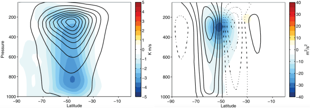
We know two types of annular modes: baroclinic (based on eddy kinetic energy, a proxy for eddy activity and an indicator of storm-track intensity) and barotropic (based on zonal mean zonal wind, representing the north-south shifts of the jet stream) (Fig. 2). The latter are usually referred to as Southern (SAM or Antarctic Oscillation) or Northern (NAM or Arctic Oscillation) Annular Mode (depending on the hemisphere), have generally quasi-barotropic (uniform) vertical structure, and impact the temperature variations, sea-ice distribution, and storm paths in both hemispheres with timescales of about 10 days. The former are referred to as BAM (baroclinic annular mode) and exhibit strong vertical structure associated with strong vertical wind shear (baroclinicity), and their impacts are yet to be determined (e.g. Thompson and Barnes 2014, Marshall et al. 2017). These two modes of variability are linked to the key processes of the midlatitude tropospheric dynamics that are involved in the growth (baroclinic processes) and decay (barotropic processes) of midlatitude storms. The growth stage of the midlatitude storms is conventionally associated with increase in eddy kinetic energy (EKE) and the decay stage with decrease in EKE.

However, recent observational studies (e.g. Thompson and Woodworth 2014) have suggested decoupling of baroclinic and barotropic components of atmospheric variability in the Southern Hemisphere (i.e. no correlation between the BAM and SAM) and a simpler formulation of the EKE budget that only depends on eddy heat fluxes and BAM (Thompson et al. 2017). Using cross-spectrum analysis, we empirically test the validity of the suggested relationship between EKE and heat flux at different timescales (Boljka et al. 2018). Two different relationships are identified in Fig. 3: 1) a regime where EKE and eddy heat flux relationship holds well (periods longer than 10 days; intermediate timescale); and 2) a regime where this relationship breaks down (periods shorter than 10 days; synoptic timescale). For the relationship to hold (by construction), the imaginary part of the cross-spectrum must follow the angular frequency line and the real part must be constant. This is only true at the intermediate timescales. Hence, the suggested decoupling of baroclinic and barotropic components found in Thompson and Woodworth (2014) only works at intermediate timescales. This is consistent with our theoretical model (Boljka and Shepherd 2018), which predicts decoupling under synoptic temporal and spatial averaging. At synoptic timescales, processes such as barotropic momentum fluxes (closely related to the latitudinal shifts in the jet stream) contribute to the variability in EKE. This is consistent with the dynamics of storms that occur on timescales shorter than 10 days (e.g. Simmons and Hoskins 1978). This is further discussed in Boljka et al. (2018).

References

Boljka, L., and T. G. Shepherd, 2018: A multiscale asymptotic theory of extratropical wave, mean-flow interaction. J. Atmos. Sci., in press.

Boljka, L., T. G. Shepherd, and M. Blackburn, 2018: On the coupling between barotropic and baroclinic modes of extratropical atmospheric variability. J. Atmos. Sci., in review.

Marshall, G. J., D. W. J. Thompson, and M. R. van den Broeke, 2017: The signature of Southern Hemisphere atmospheric circulation patterns in Antarctic precipitation. Geophys. Res. Lett., 44, 11,580–11,589.

Simmons, A. J., and B. J. Hoskins, 1978: The life cycles of some nonlinear baroclinic waves. J. Atmos. Sci., 35, 414–432.

Thompson, D. W. J., and E. A. Barnes, 2014: Periodic variability in the large-scale Southern Hemisphere atmospheric circulation. Science, 343, 641–645.

Thompson, D. W. J., B. R. Crow, and E. A. Barnes, 2017: Intraseasonal periodicity in the Southern Hemisphere circulation on regional spatial scales. J. Atmos. Sci., 74, 865–877.

Thompson, D. W. J., and J. D. Woodworth, 2014: Barotropic and baroclinic annular variability in the Southern Hemisphere. J. Atmos. Sci., 71, 1480–1493.