A new, explicit thunderstorm electrification scheme for the Met Office Unified Model

Email: Benjamin.Courtier@pgr.reading.ac.uk

Forecasting lightning is a difficult problem due to the complexity of the lightning process and how dependent the lightning forecast is on the accuracy of the convective forecast. In order to verify forecasts of lightning independently of the accuracy of the convective forecast, it can be helpful to introduce a lightning scheme that is more complex and physically representative than the simple lightning parameterisations often used in Numerical Weather Prediction (NWP).

The existing method of predicting lightning in the Met Office’s Unified Model (MetUM) uses upwards graupel flux and total ice water path, based on the method of McCaul et al. (2009). However, this method tends to overpredict the total number and coverage of lighting, particularly in the UK.

I’ve implemented a physically based, explicit electrification scheme in the MetUM in order to try and improve the current lightning forecasts. The processes involved in the scheme are shown in the flowchart in Figure 1. The electrification scheme uses the Non-Inductive Charging (NIC) process to separate charge within thunderstorms (Mansell et al., 2005; Saunders and Peck, 1998). The NIC theory states that when graupel and ice crystals collide some charge is transferred from one particle to the other. The sign and the magnitude of the charge that is transferred to the graupel particle depends on a number of parameters. It is affected by the ice crystal diameter, the velocity of the collision, the liquid water content and the temperature at which the collision occurs. Once the charge has been generated on graupel and ice or snow particles, it can be moved around the model domain and can be transferred between hydrometeor species. Charge is removed from hydrometeor species and the domain when the hydrometeors precipitate to the surface or if the hydrometeor evaporates or sublimates. Charge is transferred between hydrometeor species proportionally to the mass that is transferred. Charge is held on graupel, rain and cloud ice (or aggregates and crystals if these are included separately).

Figure 1: A flowchart showing the process and order of those processes involved within the new electrification scheme.

Once these charged hydrometeors are distributed through the cloud, they can be totalled to create a charge density distribution. From this distribution the electric field can be calculated. Then from the electric field lightning flashes can be discharged. Lightning flashes are discharged based on two thresholds, the first of these is the initiation threshold and governs where the initiation point for the lightning channel should be (Marshall et al., 1995). The second of these is a propagation threshold and governs whether or not the lightning channel can move through a grid box (Barthe et al., 2012). Lightning channels are only allowed to propagate vertically within a grid column to simplify the model structure (Fierro et al., 2013). Once the channel is created charge is neutralised along the channel, charge is removed from hydrometeor species in both the channel and the grid points immediately adjacent to the channel.

The updated charge density distribution is then used to recalculate the electric field and new flashes are discharged from any points that exceed the electric field threshold. This process keeps repeating until no new lightning flashes are discharged within the domain.

The plots in Figure 2 show the charge on graupel (a), cloud ice (b), rain (c) and the total charge (d) for a small single cell thunderstorm in the south of the UK on the 31st August 2017. It can be seen in these figure that the charge is mainly positive on cloud ice and mainly negative on graupel. The cloud ice, being less dense is lofted towards the top of the thunderstorm, while the graupel being denser generally falls towards the bottom of the storm. This creates the charge structure seen in Fig. 2d, with two positive-negative dipoles. This charge structure allows for the development of strong electric fields between the positive and negative charge centres in each dipole. If the electric field between the charge centres reaches the order of 100s kVm-1 the air can become electrically conductive, causing lightning.

Figure 2: The charge on hydrometeors in a small single-cell thunderstorm (a) shows the charge on graupel, (b) shows the charge on cloud ice, (c) shows the charge on rain and (d) shows total charge. In each plot, the outline indicated by the solid black line is the 5 dBZ reflectivity contour.

The electrification scheme was run within the operational configuration of the MetUM for a case study. The case study was a case of some organised and some single-cell, fair weather convection, on the 31st August 2017. The observations of lightning flashes are taken from the Met Office’s ATDNet lightning location system. The results of the total lighting accumulated for the entire day of the 31st August are shown in Figure 3. It can be easily seen that the existing method is producing far too much lightning compared to the observations. The new scheme is much closer to the observations.

It is an improvement, not only in the total lightning output, but also in the appearance of the lightning flash map. The scattered nature of the observations is captured by the new scheme, whereas the existing parameterisation appears to be largely producing lightning in neat, contoured paths. These paths show that the way that the existing parameterisation predicts lightning is not physically accurate and indicate the problem with the parameterisation, namely that it relies too heavily on the total ice water path. The new scheme suggests a possible improvement, in considering more explicitly the combination of graupel, liquid water and cloud ice that is vital for the production of charge and therefore lightning.

Figure 3: The total lightning flash accumulation for 31st August 2017 across the UK, (a) shows the output of the new electrification scheme, (b) shows the observed flashes, binned to match the model grid, and (c) shows the output of the existing MetUM parameterisation.

References:
Barthe, C., Chong, M., Pinty, J.-P., and Escobar, J. (2012). CELLS v1.0: updated and parallelized version of an electrical scheme to simulate multiple electrified clouds and flashes over large domains. Geoscientific Model Development, (5), 167–184.

Fierro, A. O., Mansell, E. R., MacGorman, D. R., and Ziegler, C. L. (2013). The Implementation of an Explicit Charging and Discharge Lightning Scheme within the WRF-ARW Model: Benchmark Simulations of a Continental Squall Line, a Tropical Cyclone, and a Winter Storm. Monthly Weather Review, 141, 2390–2415.

Mansell, E. R., MacGorman, D. R., Ziegler, C. L., and Straka, J. M. (2005). Charge structure and lightning sensitivity in a simulated multicell thunderstorm. Journal of Geophysical Research, 110.

Marshall, T. C., McCarthy, M. P., and Rust, W. D. (1995). Electric field magnitudes and lightning initiation in thunderstorms. Journal of Geophysical Research, 100, 7097–7103.

McCaul, E. W., Goodman, S. J., LaCasse, K. M., and Cecil, D. J. (2009). Forecasting lightning threat using cloud-resolving model simulations. Weather and Forecasting, 24(3), 709–729.

Saunders, C. P. R. and Peck, S. L. (1998). Laboratory studies of the influence of the rime accretion rate on charge transfer during crystal / graupel collisions. Journal of Geophysical Research, 103, 949–13.

An inter-comparison of Arctic synoptic scale storms between four global reanalysis datasets

Email: alexander.vessey@pgr.reading.ac.uk

The Arctic has changed a lot over the last four decades. Arctic September sea ice extent has decreased rapidly from 1980-present by approximately 3.4 million square-kilometres (see Figure 1). This has made the Arctic more accessible for human activities such as shipping, oil exploration and tourism. As Arctic sea ice is expected to continue to decline in the future, human activity in the Arctic is expected to continue to increase. This will increase the exposure to hazardous weather conditions, such as high winds and high waves, which are associated with Arctic storms. However, the characteristics of Arctic storms are currently not well understood.

Figure 1: (a) Arctic September sea ice extent from 1979-2019. (b) Spatial distribution of Arctic September sea ice extent in 1980. (c) Spatial distribution of Arctic September sea ice extent in 2019. Images have been obtained from NSIDC (2020).

One way to investigate current Arctic storm characteristics is to analyse storms in global reanalysis datasets. Reanalysis datasets combine past observations with current weather models to produce spatially and temporally homogeneous datasets, that contain atmospheric data at grid-points around the world at constant time intervals (typically every 6-hours) per day from 1979-present (for the modern, satellite-era reanalyses). Typically, a storm tracking algorithm is used to efficiently process all of the 6-hour data in the reanalysis datasets from 1979 (60,088 time steps!) to identify all of the storms that may have occurred in the past. Storms can be identified in the mean sea level pressure (MSLP) field (as low pressure systems), or in the relative vorticity field (as large rotating systems). The relative vorticity field at 850 hPa (higher in the atmosphere than the atmospheric boundary layer) is typically used so that the field is less influenced by boundary layer processes that may produce areas of high relative vorticity.

At the moment, atmospheric scientists are spoilt for choice when it comes to choosing a reanalysis dataset to analyse. There are reanalysis datasets from multiple institutions; the European Centre for Medium Range Weather Forecasts (ECMWF), the Japanese Meteorological Agency (JMA), the National Aeronautics and Space Administration (NASA), and the National Centers for Environmental Prediction (NCEP). Each institution has created their reanalysis dataset in a slightly different way, by using their own numerical weather prediction model and data assimilation systems. Atmospheric scientists also have to choose whether to use the MSLP field or 850 hPa relative vorticity field when applying their storm tracking algorithm to the reanalysis datasets.

In my recent paper, I aimed to assess Arctic storm characteristics in the multiple reanalysis datasets currently available (ERA-Interim, JRA-55, MERRA-2 and NCEP-CFSR), using a storm tracking algorithm based on 850 hPa relative vorticity and MSLP fields. Below is a short summary of some of the results from the paper.

Despite the Arctic environment changing dramatically over the last four decades, we find that there has been no change in the frequency and intensity of Arctic storms in all the reanalysis datasets compared in this study. It was found in preceding, older versions of atmospheric reanalysis datasets that Arctic storm frequency had increased from 1949-2002 (Walsh. 2008 and Sepp & Jaagus. 2011). This is in contrast with results from the modern reanalysis datasets (from this study, and Simmonds et al. 2008, Serreze and Barrett. 2008 and Zahn et al. 2018) which show no increase in Arctic storm frequency.

Across all the reanalysis datasets, some robust characteristics of Arctic storms were found. For example, the spatial distribution of Arctic storms is found to be seasonally dependent. In winter (DJF), Arctic storm track density is highest over the Greenland, Norwegian and Barents Seas, whereas in summer (JJA), Arctic storm track density is highest over and north of the Eurasia coastline (a region known as the Arctic Frontal Zone (Reed & Kunkel. 1960)) (see Figure 2). The number of trans-Arctic ships in summer is much higher than in winter, and these ships typically use the Northern Sea Route to travel between Europe and Asia (along the coastline of Eurasia). Figure 2b shows that this in fact is where most of the summer Arctic storms occur. In addition, the reanalysis datasets show that ~50% of Arctic storms have genesis in mid-latitude regions (south of 65°N) and travel northwards into the Arctic (north of 65°N). This shows that storms are a significant mechanism for transporting air from low to high latitudes.

Figure 2: Climatological track density of all Arctic storms that travel north of 65°N between 1980/81–2016/17 in (a) winter (DJF) and 1980–2017 in (b) summer (JJA) based on the ERA-Interim reanalysis. Densities have units of number per season per unit area (5° spherical cap, ≈ 10^{6} km^{2}
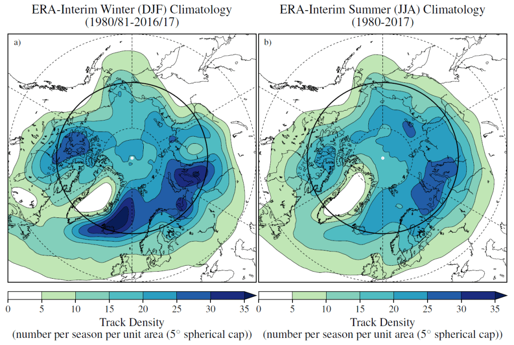
). Longitudes are shown every 60°E, and latitudes are shown at 80°N, 65°N (bold) and 50°N. Figure from Vessey at al. (2020).

In general, there is less consistency in Arctic storm characteristics in winter than in summer. This may be because in winter, the occurrence of meteorological conditions such as low level cloud, stable boundary layers and polar night that are more frequent, which are more challenging to represent in numerical weather prediction models, and for the creation of reanalysis datasets. In addition, there is a low density of conventional observations in winter, and difficulties in identifying cloud and estimating emissivity over snow and ice limit the current use of infrared and microwave satellite data in the troposphere (Jung et al. 2016).

The differences between the reanalysis datasets in Arctic storm frequency per season in winter (DJF) and summer (JJA) (1980-2017) were found to be less than 6 storms per season. On the other hand, the differences in Arctic storm frequency per season between storms identified by a storm tracking algorithm based on 850 hPa relative vorticity and MSLP were found to be 55 storms per season in winter, and 33 storms per season in summer. This shows that the decision to use 850 hPa relative vorticity or MSLP for storm tracking can be more important that the choice of reanalysis dataset.

Read more at: https://link.springer.com/article/10.1007/s00382-020-05142-4

References:

National Snow & Ice Data Centre (2019) Sea ice index. https://nsidc.org. Accessed 4 Mar 2019.

Reed RJ, Kunkel BA (1960) The Arctic circulation in summer. J. Meteorol. 17(5):489–506.

Sepp M, Jaagus J (2011) Changes in the activity and tracks of Arctic cyclones. Clim. Change 105(3–4):577–595.

Simmonds I, Burke C, Keay K (2008) Arctic climate change as manifest in cyclone behavior. J. Clim. 21(22):5777–5796.

Serreze MC, Barrett AP (2008) The summer cyclone maximum over the central Arctic Ocean. J. Clim. 21(5):1048–1065.

Vessey, A.F., Hodges, K.I., Shaffrey, L.C., Day, J.J., (2020) An inter‑comparison of Arctic synoptic scale storms between four global reanalysis datasets. Clim. Dyn., https://doi.org/10.1007/s00382-020-05142-4

Walsh, J.E., Bromwich, D.H., Overland, J.E., Serreze, M.C. and Wood, K.R., 2018. 100 years of progress in polar meteorology. Meteorological Monographs, 59, pp.21-1.

Zahn M, Akperov M, Rinke A, Feser F, Mokhov I I (2018) Trends of cyclone characteristics in the Arctic and their patterns from different reanalysis data. J. Geophys. Res. Atmos., 123(5):2737–2751.

Life on Industrial Placement

Email: holly.turner@reading.ac.uk

I finished my PhD last year, and since the start of this year I’ve been doing something rather different. Courtesy of SCENARIO DTP funding, I am doing a 3-month post-doc placement with JBA Consulting in Skipton, North Yorkshire. After spending 3.5 years researching in an academic setting, it is great to be able to apply my knowledge to real-world problems.

Working in industry has a very different feel to working in academia. The science being done has an immediate purpose for the company, rather than being done purely to extend knowledge. In the case of my placement, the work that I am doing is ultimately to benefit the end users of the product.

The field that I am now working in is rather far removed from my PhD project: I have gone from gravity waves to surface water flooding. Whilst it has been quite a steep learning curve to bring myself up to speed with the current science in this area, it is great to branch out. I would urge anyone interested in doing an industrial placement not to be put off by going outside of your subject area. You might find something else that suits you better. It might even be the best step you ever make.

The choosing and setting up of the placement has all been fairly easy for me. SCENARIO had a range of placements available and I chose the one that most interested me. I had to send an application to the company, who then called me for an interview. Once they decided to offer me the placement, SCENARIO did the setting up with both JBA and the university. All I needed to worry about was finding accommodation for the 3 months.

To anyone considering doing an industrial placement: do it! I am currently 3 weeks in and have really enjoyed it so far. Everybody has been welcoming and helpful. I felt like part of the team by the end of my first day.