The Social Metwork

Email: j.r.aylmer@pgr.reading.ac.uk

Downward trends in Arctic sea-ice extent in recent decades are a striking signal of our warming planet. Loss of sea ice has major implications for future climate because it strongly influences the Earth’s energy budget and plays a dynamic role in the atmosphere and ocean circulation.

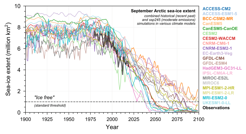
Comprehensive numerical models are used to make long-term projections of the future climate state under different greenhouse gas emission scenarios. They estimate that the Arctic ocean will become seasonally ice free by the end of the 21^st century, but there is a large uncertainty on the timing due to the spread of estimates across models (Fig. 1).

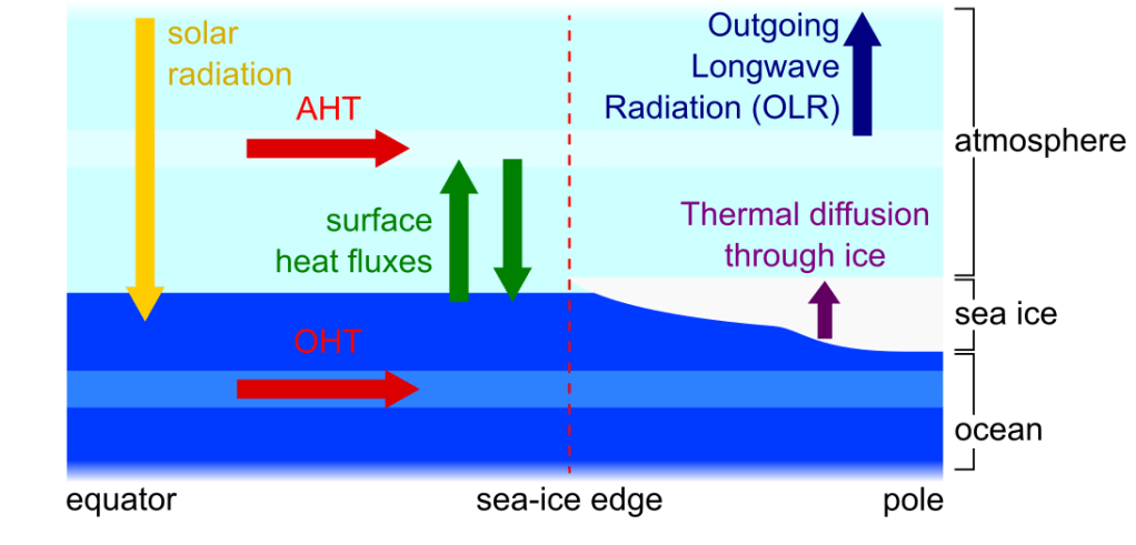
What causes this spread, and how might it be reduced to better constrain future projections? There are various factors (Notz et al. 2016), but of interest to our work is the large-scale forcing of the atmosphere and ocean. The mean atmospheric circulation transports about 3 PW of heat from lower latitudes into the Arctic, and the oceans transport about a tenth of that (e.g. Trenberth and Fasullo, 2017; 1 PW = 10¹⁵ W). Our goal is to understand the relative roles of Ocean and Atmospheric Heat Transports (OHT, AHT) on long timescales. Specifically, how sensitive is the sea-ice cover to deviations in OHT and AHT, and what underlying mechanisms determine the sensitivities?

We developed a highly simplified Energy-Balance Model (EBM) of the climate system (Fig. 2)—it has only latitudinal variations and is described by a few simple equations relating energy transfer between the atmosphere, ocean, and sea ice (Aylmer et al. 2020). The latitude of the sea-ice edge is an analogue for ice extent in the real world. The simplicity of the EBM allows us to isolate the basic physics of the problem, which would not be possible going directly with the complex output of a full climate model.

We generated a set of simulations in which OHT varies and checked the response of the ice edge. This is a measure of the effective sensitivity of the ice cover to OHT (Fig. 3a)—it is not the actual sensitivity because AHT decreases (Fig. 3b), and we are really seeing in Fig. 3a the net response of the ice edge to changes in both OHT and AHT.

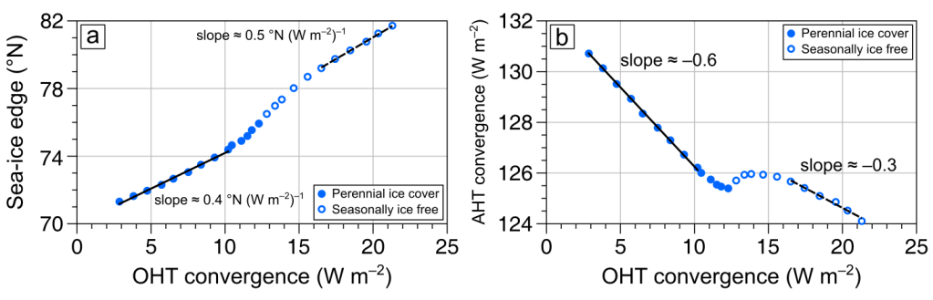
This reduction in AHT with increasing OHT is called Bjerknes compensation, and it occurs in full climate models too (Outten et al. 2018). Here, it has a moderating effect on the true impact of increasing OHT. With further analysis, we determined the actual sensitivity to be about 1.5 times the effective sensitivity. The actual sensitivity of the ice edge to AHT turns out to be about half that to the OHT.

What sets the difference in OHT and AHT sensitivities? This is easily answered within the EBM framework. We derived a general expression for the ratio of (actual) ice-edge sensitivities to OHT (s_o) and AHT (s_a):

A higher-order term has been neglected for simplicity here, but the basic point remains: the ratio of sensitivities mainly depends on the parameters B_OLR and B_down. These are bulk representations of atmospheric feedbacks and determine the efficiency of outgoing and downwelling longwave radiation, respectively. They are always positive, so the ice edge is always more sensitive to OHT than AHT.

The interpretation of this equation is simple. AHT converging over the ice pack can either be transferred to the underlying sea ice, or radiated to space, having no impact on the ice, and the partitioning is controlled by B_down and B_OLR. The same amount of OHT converging under the ice pack can only go through the ice and is thus the more efficient driver.

Climate models with larger OHTs tend to have less sea ice (Mahlstein and Knutti, 2011). We have also found strong correlations between OHT and the sea-ice edge in several of the models listed in Fig. 1 individually. Ice-edge sensitivities and B values can be determined per model, and our equation predicts how these should be related. Our work thus provides a way to investigate how much physical biases in OHT and AHT contribute to sea-ice-projection uncertainties.