High-resolution Dispersion Modelling in the Convective Boundary Layer

Lewis Blunn – l.p.blunn@pgr.reading.ac.uk

In this blog I will first give an overview of the representation of pollution dispersion in regional air quality models (AQMs). I will then show that when pollution dispersion simulations in the convective boundary layer (CBL) are run at \mathcal{O}(100 m) horizontal grid length, interesting dynamics emerge that have significant implications for urban air quality. 

Modelling Pollution Dispersion 

AQMs are a critical tool in the management of urban air pollution. They can be used for short-term air quality (AQ) forecasts, and in making planning and policy decisions aimed at abating poor AQ. For accurate AQ prediction the representation of vertical dispersion in the urban boundary layer (BL) is key because it controls the transport of pollution away from the surface. 

Current regional scale Eulerian AQMs are typically run at \mathcal{O}(10 km) horizontal grid length (Baklanov et al., 2014). The UK Met Office’s regional AQM runs at 12 km horizontal grid length (Savage et al., 2013) and its forecasts are used by the Department for Environment Food and Rural Affairs (DEFRA) to provide a daily AQ index across the UK (today’s DEFRA forecast). At such horizontal grid lengths turbulence in the BL is sub-grid.  

Regional AQMs and numerical weather prediction (NWP) models typically parametrise vertical dispersion of pollution in the BL using K-theory and sometimes with an additional non-local component so that 

F=-K_z \frac{\partial{c}}{\partial{z}} +N_l 

where F is the flux of pollution, c is the pollution concentration, K(z) is a turbulent diffusion coefficient and z is the height from the ground. N_l is the non-local term which represents vertical turbulent mixing under convective conditions due to buoyant thermals (Lock et al., 2000; Siebesma et al., 2007).  

K-theory (i.e. N_l=0) parametrisation of turbulent dispersion is consistent mathematically with Fickian diffusion of particles in a fluid. If K(z) is taken as constant and particles are released far from any boundaries (i.e. away from the ground and BL capping inversion), the mean square displacement of pollution particles increases proportional to the time since release. Interestingly, Albert Einstein showed that Brownian motion obeys Fickian diffusion. Therefore, pollution particles in K-theory dispersion parametrisations are analogous to memoryless particles undergoing a random walk. 

It is known however that at short timescales after emission pollution particles do have memory. In the CBL, far from undergoing a random trajectory, pollution particles released in the surface layer initially tend to follow the BL scale overturning eddies. They horizontally converge before being transported to near the top of the BL in updrafts. This results in large pollution concentrations in the upper BL and low concentrations near the surface at times on the order of one CBL eddy turnover period since release (Deardorff, 1972; Willis and Deardorff, 1981). This has important implications for ground level pollution concentration predicted by AQMs (as demonstrated later). 

Pollution dispersion can be thought of as having two different behaviours at short and long times after release. In the short time “ballistic” limit, particles travel at the velocity within the eddy they were released into, and the mean square displacement of pollution particles increases proportional to the time squared. At times greater than the order of one eddy turnover (i.e. the long time “diffusive” limit) dispersion is less efficient, since particles have lost memory of the initial conditions that they were released into and undergo random motion.  For further discussion of atmospheric diffusion and memory effects see this blog (link).

In regional AQMs, the non-local parametrisation component does not capture the ballistic dynamics and K-theory treats dispersion as being “diffusive”. This means that at CBL eddy turnover timescales it is possible that current AQMs have large errors in their predicted concentrations. However, with increases in computing power it is now possible to run NWP for research purposes at \mathcal{O}(100 m) horizontal grid length (e.g. Lean et al., 2019) and routinely at 300 m grid length (Boutle et. al., 2016). At such grid lengths the dominant CBL eddies transporting pollution (and therefore the “ballistic” diffusion) becomes resolved and does not require parametrisation. 

To investigate the differences in pollution dispersion and potential benefits that can be expected when AQMs move to \mathcal{O}(100 m) horizontal grid length, I have run NWP at horizontal grid lengths ranging from 1.5 km (where CBL dispersion is parametrised) to 55 m (where CBL dispersion is mostly resolved). The simulations are unique in that they are the first at such grid lengths to include a passive ground source of scalar representing pollution, in a domain large enough to let dispersion develop for tens of kilometres downstream. 

High-Resolution Modelling Results 

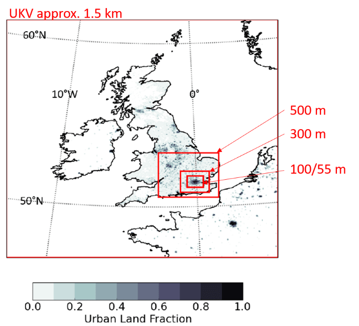
A schematic of the Met Office Unified Model nesting suite used to conduct the simulations is shown in Fig. 1. The UKV (1.5 km horizontal grid length) model was run first and used to pass boundary conditions to the 500 m model, and so on down to the 100 m and 55 m models. A puff release, homogeneous, ground source of passive scalar was included in all models and its horizontal extent covered the area of the 55 m (and 100 m) model domains. The puff releases were conducted on the hour, and at the end of each hour scalar concentration was set to zero. The case study date was 05/05/2016 with clear sky convective conditions.  

Figure 1: Schematic of the Unified Model nesting suite.

Puff Releases  

Figure 2 shows vertical cross-sections of puff released tracer in the UKV and 55 m models at 13-05, 13-20 and 13-55 UTC. At 13-05 UTC the UKV model scalar concentration is very large near the surface and approximately horizontally homogeneous. The 55 m model concentrations however are either much closer to the surface or elevated to great heights within the BL in narrow vertical regions. The heterogeneity in the 55 m model field is due to CBL turbulence being largely resolved in the 55 m model. Shortly after release, most scalar is transported predominantly horizontally rather than vertically, but at localised updrafts scalar is transported rapidly upwards. 

Figure 2: Vertical cross-sections of puff released passive scalar. (a), (b) and (c) are from the UKV model at 13-05, 13-20 and 13-55 UTC respectively. (d), (e) and (f) are from the 55 m model at 13-05, 13-20 and 13-55 UTC respectively. The x-axis is from south (left) to north (right) which is approximately the direction of mean flow. The green line is the BL scheme diagnosed BL height.

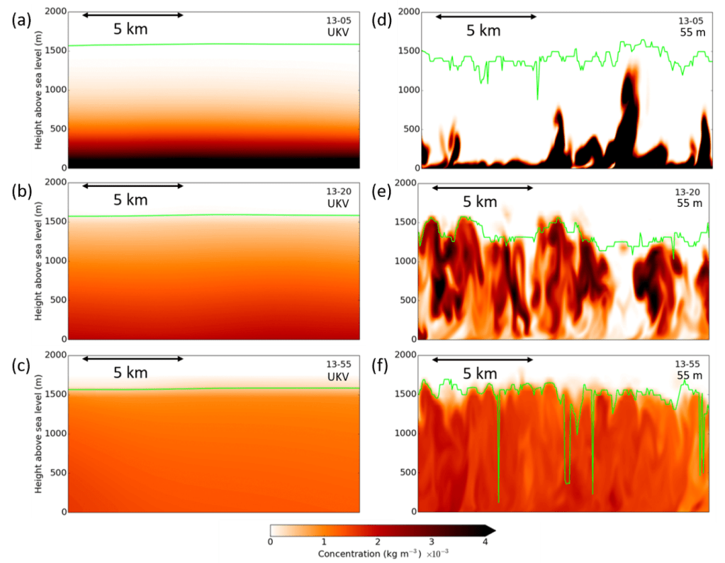
By 13-20 UTC it can be seen that the 55 m model has more scalar in the upper BL than lower BL and lowest concentrations within the BL are near the surface. However, the scalar in the UKV model disperses more slowly from the surface. Concentrations remain unrealistically larger in the lower BL than upper BL and are very horizontally homogeneous, since the “ballistic” type dispersion is not represented. By 13-55 UTC the concentration is approximately uniform (or “well mixed”) within the BL in both models and dispersion is tending to the “diffusive” limit. 

It has thus been demonstrated that unless “ballistic” type dispersion is represented in AQMs the evolution of the scalar concentration field will exhibit unphysical behaviour. In reality, pollution emissions are usually continuously released rather than puff released. One could therefore ask the question – when pollution is emitted continuously are the detailed dispersion dynamics important for urban air quality or does the dynamics of particles released at different times cancel out on average?  

Continuous Releases  

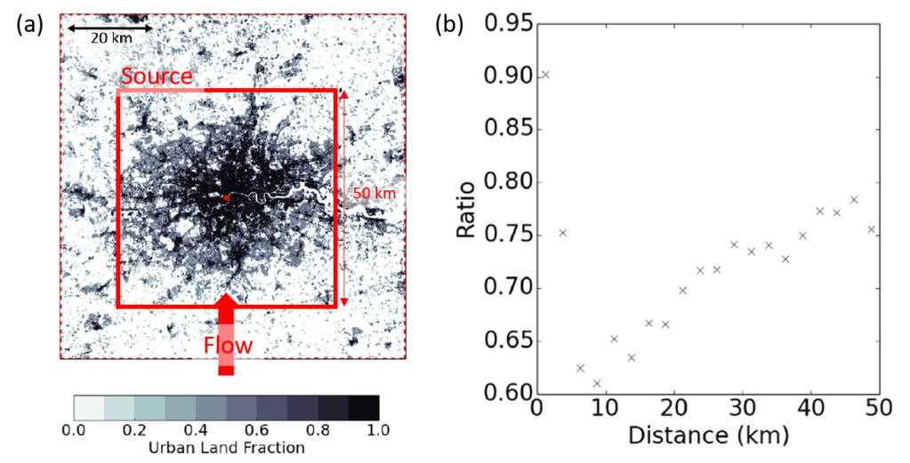
To address this question, I included a continuous release, homogeneous, ground source of passive scalar. It was centred on London and had dimensions 50 km by 50 km which is approximately the size of Greater London. Figure 3a shows a schematic of the source.  

The ratio of the 55 m model and UKV model zonally averaged surface concentration with downstream distance from the southern edge of the source is plotted in Fig. 3b. The largest difference in surface concentration between the UKV and 55m model occurs 9 km downstream, with a ratio of 0.61. This is consistent with the distance calculated from the average horizontal velocity in the BL (\approx7 ms-1) and the time at which there was most scalar in the upper BL compared to the lower BL in the puff release simulations (\approx 20 min). The scalar is lofted high into the BL soon after emission, causing reductions in surface concentrations downstream. Beyond 9 km downstream distance a larger proportion of the scalar in the BL has had time to become well-mixed and the ratio increases.  

Figure 3: (a) Schematic of the continuous release source of passive scalar. (b) Ratio of the 55 m model and UKV model zonally averaged surface concentration with downstream distance from the southern edge of the source at 13-00 UTC.

Summary  

By comparing the UKV and 55 m model surface concentrations, it has been demonstrated that “ballistic” type dispersion can influence city scale surface concentrations by up to approximately 40%. It is likely that by either moving to \mathcal{O}(100 m) horizontal grid length or developing turbulence parametrisations that represent “ballistic” type dispersion, that substantial improvements in the predictive capability of AQMs can be made. 

References 

  1. Baklanov, A. et al. (2014) Online coupled regional meteorology chemistry models in Europe: Current status and prospects https://doi.org/10.5194/acp-14-317-2014 
  1. Boutle, I. A. et al. (2016) The London Model: Forecasting fog at 333 m resolution https://doi.org/10.1002/qj.2656 
  1. Deardorff, J. (1972) Numerical Investigation of Neutral and Unstable Planetary Boundary Layers https://doi.org/10.1175/1520-0469(1972)029<0091:NIONAU>2.0.CO;2 
  1. DEFRA – air quality forecast https://uk-air.defra.gov.uk/index.php/air-pollution/research/latest/air-pollution/daqi 
  1. Lean, H. W. et al. (2019) The impact of spin-up and resolution on the representation of a clear convective boundary layer over London in order 100 m grid-length versions of the Met Office Unified Model https://doi.org/10.1002/qj.3519 
  1. Lock, A. P. et al. A New Boundary Layer Mixing Scheme. Part I: Scheme Description and Single-Column Model Tests https://doi.org/10.1175/1520-0493(2000)128<3187:ANBLMS>2.0.CO;2 
  1. Savage, N. H. et al. (2013) Air quality modelling using the Met Office Unified Model (AQUM OS24-26): model description and initial evaluation https://doi.org/10.5194/gmd-6-353-2013 
  1. Siebesma, A. P. et al. (2007) A Combined Eddy-Diffusivity Mass-Flux Approach for the Convective Boundary Layer https://doi.org/10.1175/JAS3888.1 
  1. Willis. G and J. Deardorff (1981) A laboratory study of dispersion from a source in the middle of the convectively mixed layer https://doi.org/10.1016/0004-6981(81)90001-9 

Weather Variability and its Energy Impacts

James Fallon & Brian Lo –  j.fallon@pgr.reading.ac.ukbrian.lo@pgr.reading.ac.uk 

One in five people still do not have access to modern electricity supplies, and almost half the global population rely on burning wood, charcoal or animal waste for cooking and eating (Energy Progress Report). Having a reliable and affordable source of energy is crucial to human wellbeing: including healthcare, education, cooking, transport and heating. 

Our worldwide transition to renewable energy faces the combined challenge of connecting neglected regions and vulnerable communities to reliable power supplies, and also decarbonising all energy. An assessment on supporting the world’s 7 billion humans to live a high quality of life within planetary boundaries calculated that resource provisioning across sectors including energy must be restructured to enable basic needs to be met at a much lower level of resource use [O’Neill et al. 2018]. 

Adriaan Hilbers recently wrote for the Social Metwork about the renewable energy transition (Why renewables are difficult), and challenges and solutions for modern electricity grids under increased weather exposure. (Make sure to read that first, as it provides an important background for problems associate with meso to synoptic scale variability that we won’t cover here!)  

In this blog post, we highlight the role of climate and weather variability in understanding the risks future electricity networks face. 

Climate & weather variability 

Figure 1 – Stommel diagram of the Earth’s atmosphere 

A Stommel diagram [Stommel, 1963] is used to categorise climate and weather events of different temporal and spatial scales. Logarithmic axes describe time period and size; contours (coloured areas) depict the spectral intensity of variation in sea level. It allows us to identify a variety of dynamical features in the oceans that traverse magnitudes of spatial and temporal scales. Figure 1 is a Stommel diagram adapted to describe the variability of our atmosphere.  

Microscale Smallest scales to describe features generally of the order 2 km or smaller 
Mesoscale Scale for describing atmospheric phenomena having horizontal scales ranging from a few to several hundred kilometres 
Synoptic Largest scale used to describe meteorological phenomena, typically high hundreds or 1000 km or more 

Micro Impacts on Energy 

Microscale weather processes include more predictable phenomena such as heat and moisture flux events, and unpredictable turbulence events. These generally occur at scales much smaller than the grid scale represented in numerical weather prediction models, and instead are represented through parametrisation. The most important microscale weather impacts are for isolated power grids (for example a community reliant on solar power and batteries, off-grid). Microscale weather events can also make reliable supply difficult for grids reliant on a few geographically concentrated renewable energy supplies. 

Extended Range Weather Impacts on Energy 

Across the Stommel diagram, above the synoptic scale are seasonal and intraseasonal cycles, decadal and climate variations. 

Subseasonal-to-Seasonal (S2S) forecasts are an exciting development for decision-makers across a diverse range of sectors – including agriculture, hydrology, the humanitarian sector [White et al. 2017]. In the energy sector, skilful subseasonal energy forecasts are now production ready (S2S4E DST).  Using S2S forecasts can help energy users anticipate electricity demand peaks and troughs, levels of renewable production, and their combined impacts several weeks in advance. Such forecasts will have an increasingly important role as more countries have higher renewable energy penetration (increasing their electricity grid’s weather exposure). 

Decadal Weather Cycle and Climate Impacts on Energy 

Energy system planners and operators are increasingly trying to address risks posed by climate variability, climate change, and climate uncertainty.  

Figure 2 was constructed from the record of Central England temperatures spanning the years of 1659 to 1995 and highlights the modes of variability in our atmosphere on the order of 5 to 50 years. Even without the role of climate change, constraining the boundary conditions of our weather and climate is no small task. The presence of meteorologically impactful climate variability at many different frequencies increases the workload for energy modellers, requiring many decades of climate data in order to understand the true system boundaries. 

Figure 2  – Power spectra of central England from mid 17th century, explaining variability with physical phenomena [Ghil and Lucarini 2020]

When making models of regional, national or continental energy networks, it is now increasingly common for energy modellers to consider several decades of climate data, instead of sampling a small selection of years. Figure 2 shows the different frequencies of climate variability – relying on only a limited few years of data cannot explore the extent of this variability. However significant challenges remain in sampling long-term variability and change in models [Hilbers et al. 2019], and it is the role of weather and climate scientists to communicate the importance of addressing this. 

Important contributions to uncertainty in energy system planning don’t just come from weather and climate. Variability in future energy systems will depend on technological, socioeconomic and political outcomes. Predictions of which future technologies and approaches will be most sustainable and economical are not always clear cut and easy to anticipate. A virtual workshop hosted by Reading’s energy-met group last summer [Bloomfield et al. 2020] facilitated discussions between energy and climate researchers. The workshop identified the need to better understand how contributions of all these different uncertainties propagate through complex modelling chains. 

An Energy-Meteorologist’s Journey through Time and Space 

Research is underway into tackling the uncertainties and understanding of energy risks and impacts across the spectra of spatial and temporal scales. But understanding of energy systems, and successful future planning requires decision-making involving a broad (and perhaps not fully identified) group of important technological and other factors, as well as the weather and climate impacts. It is not enough to consider any one of these alone! It is vital experts across different fields collaborate on working towards what will be best for our future energy grids. 

Tracking SDG7 – The Energy Progress Report https://trackingsdg7.esmap.org 

Why renewables are difficult – Adriaan Hilbers Social Metwork 2021 https://socialmetwork.blog/2021/01/15/why-renewables-are-difficult

O’Neill, D.W., Fanning, A.L., Lamb, W.F. et al. A good life for all within planetary boundaries https://doi.org/10.1038/s41893-018-0021-4 

Stommel, H., 1963. Varieties of oceanographic experience. Science, 139(3555), pp.572-576. https://www.jstor.org/stable/1709894

White et al (2017) Potential applications of subseasonal‐to‐seasonal (S2S) predictions https://doi.org/10.1002/met.1654 

M Ghil, V Lucarini (2020) The physics of climate variability and climate change https://doi.org/10.1103/RevModPhys.92.035002

AP Hilbers, DJ Brayshaw, A Gandy (2019) Importance subsampling: improving power system planning under climate-based uncertainty https://doi.org/10.1016/j.apenergy.2019.04.110 

Bloomfield, H. et al. (2020) The importance of weather and climate to energy systems: a workshop on next generation challenges in energy-climate modelling https://doi.org/10.1175/BAMS-D-20-0256.1 

The role of climate change in the 2003 European and 2010 Russian heatwaves using nudged storylines

Linda van Garderen – linda.vangarderen@hzg.de

During the summer of 2003, Europe experienced two heatwaves with, until then, unprecedented temperatures. The 2003 summer temperature record was shattered in 2010 by the Russian heatwave, which broke even Paleo records. The question remained, if climate change influenced these two events. Many contribution studies based on the likelihood of the dynamical situation were published, providing important input to answering this question. However, the position of low and high-pressure systems and other dynamical aspects of climate change are noisy and uncertain. The storyline method attributes the thermodynamic aspects of climate change (e.g. temperature), which are visible in observations and far more certain. 

Storylines 

All of us regularly think in terms of what if and if only. It is the human way of calculating hypothetic results in case we would have made a different choice. This helps us think in future scenarios, trying to figure out what choice will lead to which consequence. It is a tool to reduce risk by finding a future scenario that seems the best or safest outcome. In the storyline method, we use this exact mind-set. What if there was no climate change, would this heatwave be the same? What if the world was 2°C warmer, what would this heatwave have looked like then? With the help of an atmospheric model we can calculate what a heatwave would have been like in a world without climate change or increased climate change. 

In our study, we have two storylines: 1) the world as we know it that includes a changing climate, which we call the ‘factual’ storyline and 2) a world that could have been without climate change, which we call the ‘counterfactual’ storyline. We simulate the dynamical aspects of the weather extreme exactly the same in both storylines using a spectral nudging technique and compare the differences in temperatures.  To put it more precise, the horizontal wind flow is made up out of vorticity (circular movement) and divergence (spreading out or closing in). We nudge (or push) these two variables in the higher atmosphere to, on large scale, be the same in the factual and counterfactual simulations. 

Figure 1. What if we had another world where climate change did not happen? Would the heatwave have been different? Thinking in counterfactual worlds where we made (or will make) different decisions is a common way of thinking to estimate risk. Now we apply this idea in atmospheric modelling.  

European 2003 and Russian 2010 heatwaves 

Both the European heatwave in 2003 and the Russian heatwave in 2010 were extremes with unprecedented high temperatures for long periods of time. Besides, there had been little rain already from spring  in either case, which reduced the cooling effect from moisty soil to nearly nothing.  In our analysis we averaged the near surface temperatures in both storylines and compared their output to each other as well as the local climatology. Figure 2 shows the results of that averaging for the European heatwave in panel a and the Russian heatwave in panel b. We focus on the orange boxes, where the blue lines (factual storyline) and the red lines (counterfactual storyline) exceed the 5th-95th percentile climatology (green band). This means that during those days the atmosphere near the surface was uncommonly hot (thus a heatwave). The most important result in this graph is that the blue and red lines are separate from each other in the orange boxes. This means that the average temperature of the world with climate change (blue, factual) is higher than in the world without climate change (red, counterfactual).  

“Even though there would have been a heatwave with or without climate change, climate change has made the heat more extreme” 

Figure 2. Daily mean temperature at 2 meters height for (a) European summer 2003 and (b) Russian summer 2010. The orange boxes are the heatwaves, where the temperatures of the factual (blue) and counterfactual (red) are above the green band of 5th – 95th percentile climatology temperatures.  

The difference between these temperatures are not the same everywhere, it strongly depends on where you are in Europe or Russia. Let me explain what I mean with the help of Figure 3 with the difference between factual and counterfactual temperatures (right panels) on a map. In both Europe and Russia, we see that there are local regions with temperature differences of almost 0°C, and we see regions where the differences are almost 2.5°C (for Europe) or even 4°C (for Russia). A person living south from Moscow would therefore not have experienced 33°C but 29°C in a world without climate change. It is easy to imagine that such a temperature difference changes the impacts a heatwave has on e.g. public health and agriculture.  

Figure 3. Upper left: Average Temperature at 2 meter height and Geopotential height over Europe at z500 for 1-15th of August 2003, Lower left: Same as upper left but for 1-15th of Russia August 2010. Upper right: Factual minus Counterfactual average temperature at 2 meter height over Europe for 1-15th of August 2003, Lower right: same as lower left but for 1-15th of Russia August 2010. Stippling indicates robust results (all factuals are > 0.1°C warmer than all counterfactuals) 

 “The 2003 European and 2010 Russian heatwaves could locally have been 2.5°C – 4°C cooler in a world without climate change” 

We can conclude therefore, that with the help of our nudged storyline method, we can study the climate signal in extreme events with larger certainty. 

If you are interested in the elaborate explanation of the method and analysis of the two case studies, please take a look at our paper: 

van Garderen, L., Feser, F., and Shepherd, T. G.: A methodology for attributing the role of climate change in extreme events: a global spectrally nudged storyline, Nat. Hazards Earth Syst. Sci., 21, 171–186, https://doi.org/10.5194/nhess-21-171-2021 , 2021. 

If you have questions or remarks, please contact Linda van Garderen at linda.vangarderen@hzg.de

Main challenges for extreme heat risk communication

Chloe Brimicombe – c.r.brimicombe@pgr.reading.ac.uk, @ChloBrim

For my PhD, I research heatwaves and heat stress, with a focus on the African continent. Here I show what the main challenges are for communicating heatwave impacts inspired by a presentation given by Roop Singh of the Red Cross Climate Center at Understanding Risk Forum 2020.  

There is no universal definition of heatwaves 

Having no agreed definition of a heatwave (also known as extreme heat events) is a huge challenge in communicating risk. However, there is a guideline definition by the World Meteorological Organisation and for the UK an agreed definition as of 2019. In simple terms a heatwave is: 

“A period of above average temperatures of 3 or more days in a region’s warm season (i.e. all year in the tropics and in the summer season elsewhere)”  

We then have heat stress which is an impact of heatwaves, and is the killer aspect of heat. Heat stress is: 

“Build-up of body heat as a result of exertion or external environment”(McGregor, 2018) 

Attention Deficit 

Heatwaves receive low attention in comparison to other natural hazards I.e., Flooding, one of the easiest ways to appreciate this attention deficit is through Google search trends. If we compare ‘heat wave’ to ‘flood’ both designated as disaster search types, you can see that a larger proportion of searches over time are for ‘flood’ in comparison to ‘heat wave’.  

Figure 1: Showing ‘Heat waves’ (blue)  vs ‘Flood’ (red) Disaster Search Types interest over time taken from: https://trends.google.com/trends/explore?date=all&q=%2Fm%2F01qw8g,%2Fm%2F0dbtv 

On average flood has 28% search interest which is over 10 times the amount of interest for heat wave. And this is despite Heatwaves being named the deadliest hydro-meteorological hazard from 2015-2019 by the World Meteorological Organization. Attention is important if someone can remember an event and its impacts easily, they can associate this with the likelihood of it happening. This is known as the availability bias and plays a key role in risk perception. 

Lack of Research and Funding 

One impact of the attention deficit on extreme heat risk, is there is not ample research and funding on the topic – it’s very patchy. Let’s consider a keyword search of academic papers for ‘heatwave*’ and ‘flood*’ from Scopus an academic database.  

Figure 2: Number of ‘heatwave*’ vs number of ‘flood*’ academic papers from Scopus. 

Research on floods is over 100 times bigger in quantity than heatwaves. This is like what we find for google searches and the attention deficit, and reveals a research bias amongst these hydro-meteorological hazards. And is mirrored by what my research finds for the UK, much more research on floods in comparison to heatwaves (https://doi.org/10.1016/j.envsci.2020.10.021). Our paper is the first for the UK to assess the barriers, causes and solutions for providing adequate research and policy for heatwaves. The motivation behind the paper came from an assignment I did during my masters focusing on UK heatwave policy, where I began to realise how little we in the UK are prepared for these events, which links up nicely with my PhD. For more information you can see my article and press release on the same topic. 

Heat is an invisible risk 

Figure 3: Meme that sums up not perceiving heat as a risk, in comparison, to storms and flooding.

Heatwaves are not something we can touch and like Climate Change, they are not ‘lickable’ or visible. This makes it incredibly difficult for us to perceive them as a risk. And this is compounded by the attention deficit; in the UK most people see heatwaves as a ‘BBQ summer’ or an opportunity to go wild swimming or go to the beach.  

And that’s really nice, but someone’s granny could be experiencing hospitalising heat stress in a top floor flat as a result of overheating that could result in their death. Or for example signal failures on your railway line as a result of heat could prevent you from getting into work, meaning you lose out on pay. I even know someone who got air lifted from the Lake District in their youth as a result of heat stress.  

 A quote from a BBC one program on wild weather in 2020 sums up overheating in homes nicely:

“It is illegal to leave your dog in a car to overheat in these temperatures in the UK, why is it legal for people to overheat in homes at these temperatures

For Africa the perception amongst many is ‘Africa is hot’ so heatwaves are not a risk, because they are ‘used to exposure’ to high temperatures. First, not all of Africa is always hot, that is in the same realm of thinking as the lyrics of the 1984 Band Aid Single. Second, there is not a lot of evidence, with many global papers missing out Africa due to a lack of data. But, there is research on heatwaves and we have evidence they do raise death rates in Africa (research mostly for the West Sahel, for example Burkina Faso) amongst other impacts including decreased crop yields.  

What’s the solution? 

Talk about heatwaves and their impacts. This sounds really simple, but I’ve noticed a tendency of a proportion of climate scientists to talk about record breaking temperatures and never mention land heatwaves (For example the Royal Institute Christmas Lectures 2020). Some even make a wild leap from temperature straight to flooding, which is just painful for me as a heatwave researcher. 

Figure 4: A schematic of heatwaves researchers and other climate scientists talking about climate change. 

So let’s start by talking about heatwaves, heat stress and their impacts.