Already an endangered species, the Asian Elephants (Elephas maximus) continue to be increasingly threatened by habitat degradation, poaching for ivory, and conflicts with people (Sukumar 2003; Menon et al., 2017). India harbours 60% of the current Asian elephant population, but only 23% of its elephant habitats reside within protected zones while the rest are perpetually disturbed by escalating anthropogenic pressures (such as expansion of human settlements and agriculture, livestock grazing and fuelwood gathering) and economic activities (mining, construction of road-railway networks etc.). Habitat degradation contributes to increasing elephant encounters with people and triggering human-elephant conflict (HEC). The conflict scenario in India escalates day by day gaining in severity and frequency. In the four-year period between 2015 and 2018 alone, it had caused deaths of around 2,400 people and 490 elephants and annually, 0.5 million households suffered due to crop loss by elephant raiding from 2000 through 2010 (MOEF 2012; MoEF & CC, 2018). Elephants have the capacity to adapt to a mosaic of natural and modified habitats and their preference of habitat selection is often determined by the landscape composition as well as space and resource availability (such as vegetation and water). Thus, comprehension of elephants’ space-use with respect to their distribution is crucial for managing human-wildlife coexistence. We conducted our study on the space-use of elephants in the Keonjhar forest division in eastern India, where several hundreds of elephants have been killed as a result of electrocution, road-train mishaps, poaching and HEC.
Figure. 1: Pattern of estimated elephant occupancy, which was evaluated using the top model for occupancy probability. Keonjhar forest division has seven forest ranges (Barbil, Bhuiyan-Juang Pihra (BJP), Champua, Ghatgaon, Keonjhar, Patna and Telkoi). Five elephant habitat cores (light blue color polygon) were identified and named as CFR, KFR, BFR, GFR and TFR
We used a popular species distribution technique called occupancy modeling, which analyzed the histories of elephant presence or absence on the survey sites (MacKenzie et al. 2017) to estimate the probability of elephant presence and underlying driving factors. For occupancy modeling, we used elephant GPS location at different sites along with anthropogenic and environmental variables, including climate variables such as precipitation data derived from monthly rain gauge data and mean annual temperature from MODIS-MOD11A1. Sentinel-2A satellite images were very helpful for extracting variables such as forests, cropland and settlements.
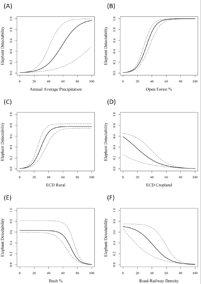
We observed elephant occupancy in 43% of the study region (about 2710 km2) (Figure 1) and occupancy was found to be higher in the regions with over 40% open forest cover (Figure 2B). It is easy to believe that a mega herbivore species like the elephants would prefer dense forests with minimum anthropogenic disturbances. However, we were surprised to find that elephants were actually drawn towards forests in human dominated landscapes with multiple land-use activities, over relatively intact forests (Sitompul et al., 2013; Huang et al. 2019). Scrubs and grasses, which are a primary forage of elephants, can grow easily in open forests as they receive better space and light conditions. Thus, open forests are the strongest variable influencing elephant occupancy, which specifically plays an important role in providing food and shelter for elephants as well as in their thermoregulation.
Figure. 2: Relationships between elephant detectability and the influential covariates
Furthermore, train-vehicle collisions have been one of the major causes of elephant mortality through the years (Jha et al., 2014; Dasgupta & Ghosh, 2015), so we evidenced a lower elephant occupancy in the regions with denser transportation networks (Figure. 2F). Even though crops are not natural forage for elephants, they preferred crops over grazing on natural forage, due to higher accessibility, palatability and nutrition (Sukumar, 1990; Campos-Arceiz et al., 2008). Thus, elephant detectability near croplands was relatively high.
When it comes to climate variables, we found a positive influence of precipitation on elephant detection, which was contrary to a study conducted in an extremely wet landscape of Southern India, that found how precipitation was the least influential covariate. However, we believe that favourable rainfall conditions improved water availability, while also increasing the productivity of deciduous forests with an abundance of palatable trees (Kumar et al., 2010; Jathanna et al., 2015), which attracted more elephants to these regions in the study area. Therefore, it is reasonable that variations in precipitation will be immediately reflected in the elephants’ space-use as rain-driven vegetation can prompt highly opportunistic elephant movement patterns.
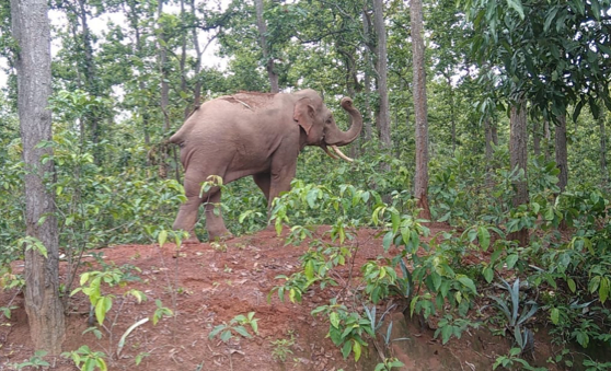
Elephant sighting in an open forest
Elephant sighting in croplands
It is very challenging to demarcate exclusive regions for people and elephants within the varying landscapes of India where both human and elephant populations are high. However, owing to the presence of areas which are more frequently used by elephants such as the five habitat cores that we identified in our study (Figure 1), we can conclude that this region still has the potential to support a significant elephant population (Tripathy et al., 2021). Hence, for efficient landscape management and planning it is critical to understand the spatial factors that potentially influence the preference of space-use by elephants in this region which will in turn ensure peaceful coexistence between elephants and people while also facilitating elephant conservation strategies.
The National Centre for Earth Observation (NCEO) is a distributed NERC centre of over 100 scientists from UK universities and research organisations (https://www.nceo.ac.uk). Last month NCEO launched a new and exciting headquarters, the Leicester Space Park. After the launch, researchers from various institutions with affiliations to NCEO were invited to a forum at the new HQ. This was an introductory workshop in Machine Learning and Artificial Intelligence. We were both lucky enough to attend this in-person event (with the exception of a few remote speakers)!
As first year PhD students, we should probably introduce ourselves:
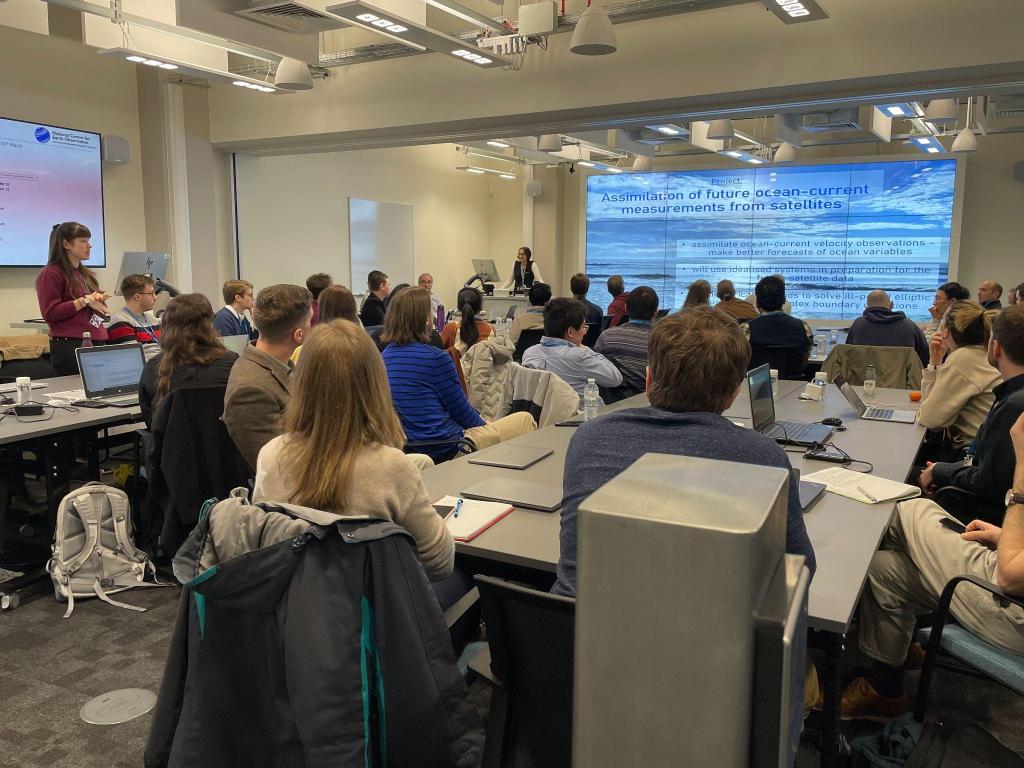
Laura – I am a Scenario student based in the Mathematics department, my project is ‘Assimilation of future ocean-current measurements from satellites’. This will involve applying data assimilation to assimilate ocean-current velocities in preparation for data from future satellites. My supervisor is also the training lead and co-director of Data Assimilation at NCEO. I was thrilled to be able to attend this forum to learn new techniques that can be used in earth observation.
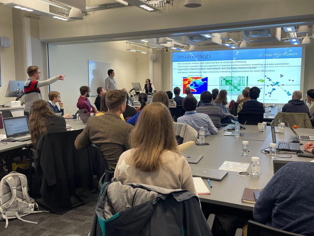
Ieuan – I am a Scenario Associate based in the Meteorology department. My project is titled ‘Complex network approach to improve marine ecosystem modelling and data assimilation’. In my work, I hope to apply some complex-network-informed machine learning techniques to predict concentrations of the less well observable nutrients in the ocean, from the well observable quantities – such as phytoplankton! As a member and fundee of NCEO, I was excited to see a training event on offer that was highly relevant to my project.
Machine Learning (ML) and Artificial Intelligence (AI) are often thought of as intimidating and amorphous topics. This fog of misconceptions was quickly cleared up, however, as the workshop provided a brilliant, fascinating and well-structured introduction into how these fields can be leveraged in the context of earth observation.
Introduction to NCEO
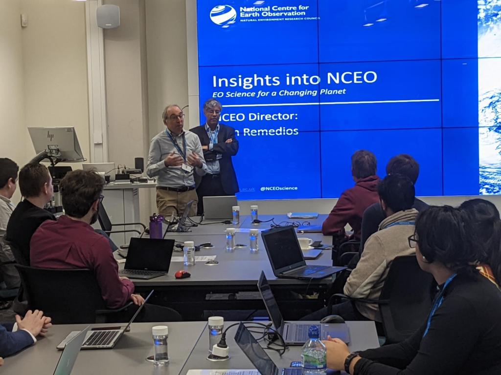
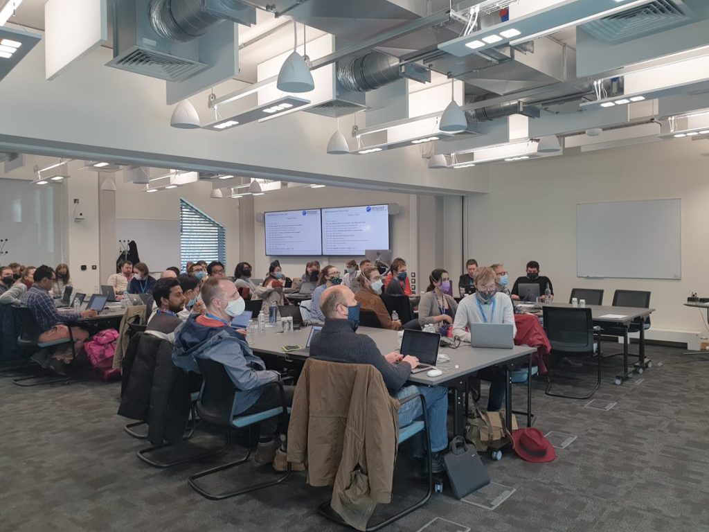
The forum began bright and (very) early on Wednesday morning at the Leicester Space Park. Our first day of ML training began with an introduction to NCEO by director – John Remedios, and training lead – Amos Lawless. We each had the opportunity to introduce ourselves and our research in a quick two-minute presentation. This highlighted the variety in both background and experience in an entirely positive way! As well as benefiting directly from the training itself, we enjoyed being in a room full of enthusiastic people with knowledge and niches aplenty.
Introducing ourselves and our research
Next, we had a talk from Sebastian Hickman, a PhD student at the University of Cambridge, who introduced his work on using ML with satellite imagery to detect tall-tree-mortalities in the Amazonian rainforest. A second talk was given by Duncan Watson-Parris from the University of Oxford on using ML to identify ship tracks from satellite imagery. These initial talks immediately got us thinking about the different ways in which ML could be used within the realm of earth science. The second day we also had talks from ESA’s Φ-lab, on a whole host of different uses for AI in earth observation.
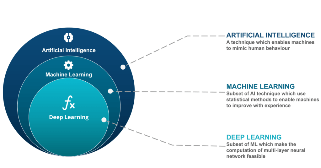
To begin our ML training, members of NEODAAS (NERC Earth Observation Data Acquisition and Analysis Service), David Moffat and Katie Awty-Carroll, led us through an introduction into ML and AI, its uses and importance in modern scientific context. The graphic below – presented by David and Katie – makes a digestible distinction between some commonly conflated terms in the subject area:
AI vs ML vs DL*
The discussion on the limitations and ‘bottlenecks’ of ML was of particular interest, it highlighted the numerous considerations to be made when developing an ML solution. For example, the subset of data used to train a model should ideally be representative of the entire system, avoiding or at least acknowledging the potential biases introduced by: human-preferences in selecting and filtering training data; the method of data collection method; the design of the ML techniques used; and how we interpret the outputs. While this may seem obvious at first, it is certainly not trivial. There are high-profile and hotly-debated examples of AI being used in the real-world where biases have led to significant human-affecting consequences. (https://sitn.hms.harvard.edu/flash/2020/racial-discrimination-in-face-recognition-technology) (https://www.ncbi.nlm.nih.gov/pmc/articles/PMC6875681)
We were prompted to consider these ethical questions and the efficacy of ML in the context of earth science: Which problems does ML help us solve and, perhaps more importantly, which problems are we willing to entrust it with?
A fun exercise you can try for yourself: search for images of a given profession in your search engine of choice. See if you can identify any patterns or biases in what may have been included or even excluded from the selected results!
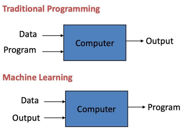
We then began the practical sessions which all fell within the broad umbrella of ML. This required a slight mindset shift from traditional programming as, even from a top-down perspective, the way we approached problems was completely different:
Figure: Traditional Programming vs Machine Learning*
We were given jupyter notebooks to work on three separate practical’s; random forest classification, neural network for regression, and convolutional neural networks. Each showed a different application and use-case of ML, giving us more ideas on how it could potentially be implemented into our own research. Adjacent to this, we were given a workflow task to think about over the two days: how could we use ML in our own projects? At the end of the second day we each presented our ideas and were given feedback. This helped ground the talks with an ongoing focus to relate new knowledge back to our own varied fields; allowing the workshop to elegantly handle the variety and promote the actual use of the skills in our own work.
The forum was academically challenging but it was also great fun! Surrounding the concentrated days of learning, the forum offered us plenty of chances to connect with others. We were given a tour of the Space Park, an impressive space you could say was out of this world. The evening activities, bowling and shuffleboard, had a great atmosphere too!
NCEO Forum Delegates 2022 outside Leicester Space Park
By the end of the event, the interest and enthusiasm of the attendees had been effectively transformed into new understanding and conversation – which is unsurprising considering the increasing relevance ML is gaining in the field of earth science. Further to this, making connections over the pandemic has been difficult, so we felt extremely fortunate that we were able to meet in person.
Laura– The forum was an exciting insight into a field I had no experience in. Although my immediate work is focused on the application of data assimilation to ocean measurements, which does not directly relate to ML at the moment, data assimilation has high potential to overlap with ML .The forum has furthered my understanding of fields that surround the focal point of my research. In turn, this has helped me gain a more well-rounded knowledge base, opening doors to new directions my research could take.
Ieuan – The forum has certainly given me many new avenues to explore when approaching the intended application of ML in my work, perhaps starting simple with a neural network for multivariate regression and expanding from there. The hands-on practicals were a valuable opportunity for practice and a great chance for some informal discussion on the details of ML implementation with my peers. Moreover, the event has equipped us with the skills to effectively engage with other academics when they present ML-based work – which is something I would love to do in future events!
We both hope there will be more NCEO workshops like this in the future, perhaps an event or meetup that focuses on the intersection of ML and data assimilation, as these topics resonate with us both. We’d like to thank the NEODAAS staff from PML for leading the training and Uzma Saeed for organising the forum. It was a fun and engaging experience that we are grateful to have taken part in and we would encourage anyone with the opportunity to learn about ML to do so!
* Graphics were provided by the NEODAAS slides used at the NCEO forum
Due to lockdowns and travel restrictions since 2020, networking opportunities in science have been transformed. We can expect to see a mix of virtual and hybrid elements persist into the future, offering both cost-saving and carbon-saving benefits.
The MeteoXchange project aims to become a new platform for young atmospheric scientists from all over the world, providing networking opportunities and platforms for collaboration. The project is an initiative of German Federal Ministry of Education and Research, and research society Deutsche Forschungsgesellschaft. Events are conducted in English, and open to young scientists anywhere.
ECS Conference
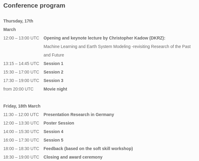
This year marked the first ever MeteoXchange conference, which took place online in March 2022. The ECS (early career scientists) conference took place over two days, on gather.town. An optional pre-conference event gave the opportunity for new presenters to work on presentation skills and receive feedback at the end of the main conference.
Figure 1: Conference Schedule, including a keynote on Machine Learning and Earth System Modelling, movie night, and presenter sessions.
Five presenter sessions were split over two days, with young scientists sharing their research to a conference hall on the virtual platform gather.town. Topics ranged from lidar sensing and reanalysis datasets, to cloud micro-physics and UV radiation health impacts. I really enjoyed talks on the attribution of ‘fire weather’ to climate change, and machine learning techniques for thunderstorm forecasting! The first evening concluded with a screening of documentary Picture a Scientist.
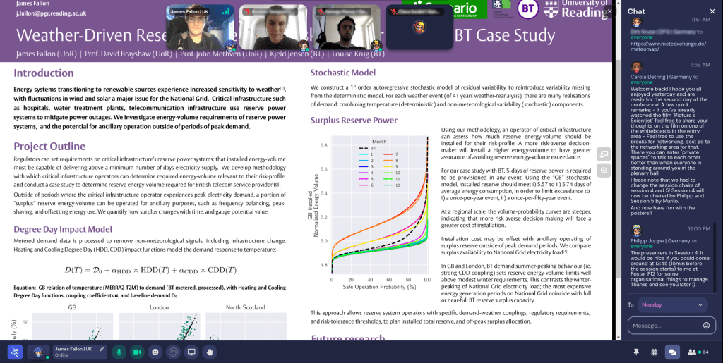
During the poster session on the second day, I presented my research poster to different scientists walking by my virtual poster board. Posters were designed to mimic the large A2 printouts seen at in-person events. Two posters that really stood out were a quantification of SO2 emissions from Kilauea volcano in Hawaii, and an evaluation of air quality in Cuba’s Mariel Bay using meteorological diagnostic models combined with air dispersion modelling.
Anticipating that it might be hard to communicate on the day, I added a lot of text to my poster. However, I needn’t have worried as the virtual platform worked flawlessly for conducting poster Q&A – the next time I present on a similar platform I will try to avoid using as much text and instead focus on a more traditional layout!
Figure 2: During the poster session, I presented my research on Reserve-Power systems – energy-volume requirements and surplus capacity set by weather events.
By the conference end, I got the impression that everyone had really enjoyed the event! Awards were given for the winners of the best posters and talks. The ECS conference was fantastically well organised by Carola Detring (DWD) and Philipp Joppe (JGU Mainz), and a wonderful opportunity to meet researchers from around the world.
MeteoMeets
Since July 2021, MeteoXchange have held monthly meetups, predominantly featuring lecturers and professors who introduce research at their institute for early career scientists in search of opportunities!
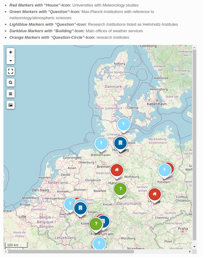
The opportunities shared at MeteoMeets are complemented by joblists and by the MeteoMap: https://www.meteoxchange.de/meteomap. The MeteoMap lists PhD and postdoc positions across Germany, neatly displayed with different markers depending on the type of institute. This resource is currently still under construction.
Figure 3: The MeteoMap features research opportunities in Germany, available for early career researchers from across the world.
Travel Grants
One of the most exciting aspects of the MeteoXchange project is the opportunity for international collaboration with travel grants!
The travel funds offered by MeteoXchange are for two or more early career scientists in the field of atmospheric sciences. Students must propose a collaborative project, which aims to spark future work and networking between their own institutions. If the application is successful, students have the opportunity to access 2,500€ for travel funds.
Over the last two weeks of April, I will be collaborating with KIT student Fabian Mockert on “Dunkelflauten” (periods of low-renewable energy production, or “dark wind lulls”). Dunkelflauten, especially cold ones, result in high electricity load on national transmission networks, leading to high costs and potentially cause a failure of a fully renewable power system doi.org/10.1038/nclimate3338. We are collaborating to use power system modelling to better understand how this stress manifests itself. Fabian will spend two weeks visiting the University of Reading campus, meeting with students and researchers from across the department.
Get Involved
The 2022 travel grant deadline has already closed; however, it is hoped that MeteoXchange will receive funding to continue this project into future years, supporting young researchers in collaboration and idea-exchange.
To get involved with the MeteoMeets, and stay up to date on MeteoXchange related opportunities, signup to the mailing list!
“Quo Vadis”, Latin for “Where are you marching?”, is an annual event held in the Department of Meteorology in which mostly 2nd year PhD students showcase their work to other members in the department. The event provides the opportunity for students to present research in a professional yet friendly environment. Quo Vadis talks usually focus on a broad overview of the project and the questions they are trying to address, the work done so far to address those questions and especially an emphasis on where ongoing research is heading (as the name of the event suggests). Over the years, presenters have been given constructive feedback from their peers and fellow academics on presentation style and their scientific work.
This year’s Quo Vadis was held on 1st March 2022 as a hybrid event. Eleven excellent in-person talks covering a wide range of topics were delivered in the one-day event. The two sessions in the morning saw talks that ranged from synoptic meteorology such as atmospheric blocking to space weather-related topics on the atmosphere of Venus, whereas the afternoon session had talks that varied from storms, turbulence, convection to energy storage!
Every year, anonymous staff judges attend the event and special recognition is given to the best talk. The winning talk is selected based on criteria including knowledge of the subject matter, methods and innovativeness, results, presentation style and ability to answer questions after the presentation. This year, the judges were faced with a difficult decision due to the high standard of cutting-edge research presented in which presenters “demonstrated excellent knowledge of their subject matter, reached conclusions that were strongly supported by their results, produced well-structured presentations, and answered their questions well.”
This year’s Quo Vadis winner is Natalie Ratcliffe. She gave an impressive presentation titled “Using Aircraft Observations and modelling to improve understanding of mineral dust transport and deposition processes”. The judging panel appreciated the combination of observations and modelling in her work and were impressed by her ability to motivate and communicate her findings in an engaging way. In addition to the winner, three honourable mentions were made this year. These went to Hannah Croad, Brian Lo and James Fallon whose talks were on arctic cyclones, using radar observations in the early identification of severe convection and weather impacts on energy storage respectively.
Being the first in-person event for a long time, Quo Vadis 2022 was a huge success thanks to our organisers Lauren James and Elliott Sainsbury. Having run for 30 years, Quo Vadis remains a highlight and an important rite of passage for PhD students in the meteorology department. Having presented at this year’s event, I found that summarising a year’s worth of research work in 12 minutes and making it engaging for a general audience is always a challenge. The audience at any level attending the event would at the very least appreciate the diversity of the PhD work within an already specialised field of meteorology. Who knows how Quo Vadis will evolve in the coming 30 years? Long may it continue!
Hello readers, and a happy new year to you all! (ok we’re a bit late on that one… but regardless we both wish you a great start to 2022!)
We have really enjoyed reading and publishing all of the posts submitted over the last year, and following all of the research conducted by PhD students in the Reading department of Meteorology. There have been posts on conferences, papers, visitors, and much more, finishing with the heralded Met dept. Pantomime!
Thank you to everyone who has contributed to the Social Metwork over this past year. We are really looking forward to new submissions this term – and whether you are a veteran contributor or have never written for a blog before, we really encourage you to get in touch and write for us 🙂
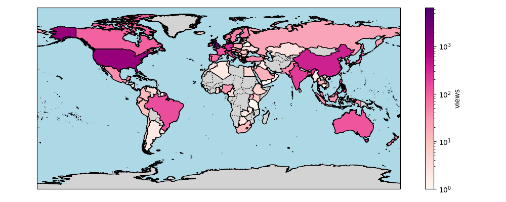
In the last year, the blog has had over 7900 visitors from all over the world!
Map of visitors to the social metwork in 2021
Compared to 2020 we have seen Brazil and Australia enter the top 10 highest number of readers at 144 and 118 views respectively. And leading with the top 3 number of views are United Kingdom (6495), United States (1134) and China (361).
In case you missed any posts, or want to look through your favourites, here are all of the posts from 2021:
Charlie Suitters – c.c.suitters@pgr.reading.ac.uk Hannah Croad – h.croad@pgr.reading.ac.uk Isabel Smith – i.h.smith@pgr.reading.ac.uk Natalie Ratcliffe – n.ratcliffe@pgr.reading.ac.uk
The pantomime has been one of the highlights of the year for the last 3 decades in the Met department. This is put on by the PhD students, and usually performed in person at the end of the Autumn term. Despite the ongoing COVID-19 pandemic, the panto is going from strength to strength, with a virtual instalment in 2020, and adapting to the hybrid format this year. It’s amazing to see the department tradition continue.
This year the four of us (Charlie Suitters, Hannah Croad, Isabel Smith and Natalie Ratcliffe) agreed to organise the panto. It was clear that the panto this year would need to cater for both people joining in person and virtually, and with the lingering uncertainty of the covid situation in the UK, we came to a group decision to pre-record the performance in advance. This would provide the best viewing experience for everyone, and provided a contingency if the covid situation worsened. In hindsight, this was a good decision.
This year’s panto was called Semi-Lagrangian Rhapsody, an idea based on the story of the band Queen. On Thursday 9th December 2021 we screened our pre-recorded pantomime in a hybrid format, with people watching both in the Madejski lecture theatre on campus and at home via Teams (probably in their pyjamas). Our story begins with our research group, Helen Dacre, Keith Shine, and Hilary Weller, on the lookout for a fourth member. In an episode of Mets Factor, the group sit through terrible auditions from Katrina and the Rossby Waves, Wet Wet Wet, the Weather Girls and Jedward (comprised of John Methven and Ed Hawkins), before finally stumbling upon Thorwald Stein (aka Eddy Mercury). The research group QUEEN (Quasi-Useful atmosphEric Electricity Nowcasting) is formed. Inspired by an impromptu radiosonde launch on the MSc field trip and skew-Ts (Chris knows!), QUEEN develop a Semi-Lagrangian convection scheme for lightning. Our narrator, SCENARIO administrator Wendy Neale, tells the story of the ups and downs of QUEENs journey, culminating in a presentation of their Semi-Lagrangian Rhapsody to the world at the AMS conference.
Natalie suggested the idea for the panto, and we all agreed that it was a great idea – especially with the potential for lots of Queen songs! Once we had our storyline, next came the script writing. This was a daunting task, but working as a team we managed to produce a decent first draft in one intensive script-writing week, full of amazing terrible meteorology puns. Whilst writing the script we decided on the best Queen songs for the plot (and for reasons that we cannot explain/remember, a Rebecca Black song too). Now it was time to alter the lyrics, which was a lot of fun! Only once we had written the songs did we actually consider the complexity of Freddie Mercury’s voice and how we, a bunch of non-musically talented PhD students, were going to attempt to do these songs any justice. It was too late to go back though, and we had to break the news to the band. Thankfully they were up to the challenge!
From week 6 onwards, we were able to start recording scenes; we were lucky that we were able to film in-person in and around the Met Department. We were still able to include students who weren’t in Reading at the time by writing in virtual parts into the panto. This worked perfectly well given the very hybrid nature of life currently anyway.
Like last year, we wanted to start earlier as we knew that we needed to be finished at least a week – preferably more – before the big night to give time to edit everything in time (there were still a couple of late nights just before the big night). The final late night session did lead to the incredible slow-mo shot of Nicki Robinson (Charlie) turning around in Bohemian Rhapsody, so there is something that can be said about late-night-induced-insanity!
Come week 10, we had nearly finished all of our filming and only had the songs left to record. We arrived at the London Road music rooms not yet having heard any of the band’s rehearsals. They sounded amazing. Many thanks to James and Gabriel who had been organising the band throughout the term. Then we started singing and immediately reduced the quality! But with a bit of practice around the piano, we started to improve, though the beginning of Bohemian Rhapsody was still a little questionable… With lots of pizza, we managed to record all of the songs in two nights! The band did an amazing job to put up with our musical incompetence (we are so very sorry).
Over the next week, our three video editors worked hard to put the whole panto together and I hope you agree that they did a good job. This all led up to the big night where we were able to offer a small pre-panto reception in the Met coffee room before the panto started (somewhat attempting to mirror the normal pre-panto buffet). Apart from one slip up in scene 4 (my apologies hehe – Natalie), the screening went nearly perfectly with very few hybrid IT complications. Additionally, we had the return of an in-person performance of Mr Mets by our own Jon Shonk, and a heartwarming singing performance from the staff, organised by Chris Holloway and Keith Shine. Not only were we gifted this, but we were able to enjoy an in-person after-party in the coffee room with DJ Shonk. Of course there were a few Queen songs scattered in the mix, though we realised we struggled to remember the original lyrics and were only able to sing the panto versions! Following the story of Queen may have been a good idea, but have we forever ruined their songs for ourselves forever now? Quite possibly…
And on that bombshell, we’d like to thank everyone who was involved in this panto, whether that be those who we convinced to act, sing, play in the band, help organise the event or even just come along to the screening. The whole process of creating this panto was exhausting, but so incredibly fun. I (Natalie) am so glad I did it and had a great time, but I now understand the ‘I’ve done my time’ sentiment of the previous organisers. (Hannah) Organising the panto was a lot of work, but so much fun (see bloopers). This has been a really rewarding experience, to see it all come together on the night, and to contribute to a fantastic department tradition.
This year we sold tickets for the in-person showing and asked for donations to the David Grimes Trust from those viewing from home. Thank you to everyone who has already donated. Your generosity is greatly appreciated. We have managed to raise £170 for the David Grimes Trust. If you would like to donate still, please find our email with details on how to do so from Hannah Croad.
Thank you to everyone who watched Semi-Lagrangian Rhapsody on Thursday, we hope you had a fun evening whether you watched at home or in-person!
Convective self-aggregation is the process by which initially randomly scattered convection becomes spontaneously clustered in space despite uniform initial conditions. This process was first identified in numerical models, however it is relevant to real world convection (Holloway et al., 2017). Tropical weather is dominated by convection, and the degree of convective aggregation has important consequences for weather and climate. A more organised regime is associated with reduced cloudiness, increased longwave emission to space (Bretherton et al., 2005), and a higher frequency of long-lasting extreme precipitation events (Bao and Sherwood, 2019).
Because of its relevance to weather and climate, self-aggregation has been the focus of many recent studies. However, there is still much debate as to the processes that cause aggregation. There is great variability in the rate and degree of aggregation between models, and there remains uncertainty as to how aggregation is affected by climate change (Wing et al., 2020). Previous studies have shown that feedbacks between convection and shortwave & longwave radiation are key drivers and maintainers of aggregation (e.g. Wing & Cronin 2016), and that interactive radiation in models is essential for aggregation to occur (Muller & Bony 2015).
This blog summarises results from the first paper from my PhD (Pope et al., 2021), where we develop and use a framework to analyse how radiative interactions with different cloud types contribute to aggregation. We analyse self-aggregation within a set of three idealised simulations of the UK Met Office Unified Model (UM). The simulations are configured in radiative-convective equilibrium over three fixed sea surface temperatures (SSTs) of 295, 300 and 305 K. They are convection permitting models that are 432 × 6048 km2 in size with a 3 km horizontal grid spacing. The simulations neglect the earth’s rotation, so they approximately represent convection over tropical oceans within a warming climate.
Our analysis framework is based on that used in Wing and Emanuel (2014) which uses the variance of vertically-integrated frozen moist static energy (FMSE) as a measure of aggregation. FMSE is a measure of the total energy an air parcel has if all the water (vapour and frozen) was converted to liquid, neglecting its velocity. Variations in vertically-integrated FMSE come from perturbations in temperature and humidity. As aggregation increases, moist regions get moister and dry regions get drier, so the variance of vertically-integrated FMSE increases.
The problem with using FMSE variance as an aggregation metric is that it is highly sensitive to SST. A warmer atmosphere can hold more water vapour via the Clausius-Clapeyron relationship. This means there is a greater difference in FMSE between the moist and dry regions for higher-SST simulations, so the variance of FMSE is typically much greater for higher SSTs. To account for this problem, we normalise FMSE between hypothetical upper and lower limits which are functions of SST. This gives a value of normalised FMSE between 0 and 1.
Wing and Emanuel (2014) derive a budget equation for the rate of change of FMSE variance which shows how different processes contribute to aggregation. By rederiving their equation for normalised FMSE , we get:
where is vertically-integrated FMSE, and are the net atmospheric column longwave and shortwave heating rates, is the surface enthalpy flux, made up of the surface latent and sensible heat fluxes, and is the horizontal divergence of the flux. Primes () indicate local anomalies from the instantaneous domain mean. The subscript () denotes a normalised variable which is the original variable divided by the difference between the hypothetical upper and lower limits of . The equation shows that the rate of change of variance (left hand side term) is driven by interactions between anomalies and anomalies in normalised net longwave heating, shortwave heating, surface fluxes and advection.
Figure 1: Hovmöller plots of normalised FMSE for each SST
Figure 2: (a) Time series of vertically-integrated FMSE variance, (b) Time series of normalised vertically-integrated FMSE variance for each SST
We use the variance of as our aggregation metric. Hovmöller plots of are shown in Figure 1 for each of our SSTs. In these plots, is averaged along the short axis of our domains. The plots show how initially randomly-distributed convection organises into bands which expand until the point where there are 4 to 5 quasi-stationary bands of moist convective regions separated by dry subsiding regions. This demonstrates that once our domains become fully-aggregated, the degree of aggregation appears similar. Figure 2a shows time series of each of the variance of , and shows that the variance of non-normalised is ~4 times greater for our 305 K simulations compared to our 295 K simulation. Figure 2b shows time series of the variance of . From this, we can see the convection aggregates faster as SST increases, yet the degree of aggregation remains similar via this metric once the convection is fully aggregated. Values of variance around 10-4 or lower correspond to randomly scattered convection, whereas values greater that 10-3 are associated with strongly aggregated convection.
Figure 3: Maps of (a) cloud condensed water path, (b) vertically-integrated FMSE anomaly, (c) longwave heating anomaly, (d) shortwave heating anomaly. Snapshots at day 100 of the 300 K simulation.
To understand the processes contributing to aggregation, we have to look to Equation 1. We mainly focus on the two radiative terms on the right hand side. The terms show that regions in which the radiative anomalies and the anomalies have the same sign contribute to aggregation. We can start to get an intuitive understanding of this concept by looking at maps of these variables. Figure 3b-d show maps of , and . We can see and are closely correlated since is mainly determined by the shortwave absorption by water vapour. Clouds have little effect on the shortwave heating rates, with ~90% of the shortwave heating rate in cloudy regions being due to absorption by water vapour. is closely linked to cloud condensed water path (Figure 3a). This is because the majority of our clouds are high-topped clouds which, due to their cold cloud tops, are able to prevent longwave radiation escaping to space, so they are associated with positive longwave heating anomalies.
The sensitivity of the budget terms to both aggregation and SST can be seen in Figure 4. This figure is made by creating 50 bins of variance and then averaging the budget terms in space and time for each bin and for each SST. Where the terms are positive, they are helping to increase aggregation. Where they are negative, the terms are opposing aggregation. The terms tend to increase in magnitude since every term has as a factor, which increases with aggregation by definition.
Figure 4: Terms in Equation 1 vs normalised FMSE variance for each SST
In general, we find the longwave term is the dominant driver of aggregation, being insensitive to SST during the growth phase of aggregation. Once the aggregation is mature, the longwave term remains the dominant maintainer of aggregation, however its contribution to aggregation maintenance decreases with SST. The shortwave term is initially small at early times but becomes a key maintainer of aggregation within highly-aggregated environments. This is because humidity variations are initially small, so there is little variation in shortwave heating. Once the convection is aggregated, moist regions are very moist and dry regions are very dry, so there is a large difference in shortwave heating between moist and dry regions. The variations in shortwave heating remain very similar with SST, meaning shortwave heating anomalies contribute the same amount to non-normalised variance. Therefore, shortwave heating contributes less to aggregation at higher SSTs because they contribute to a smaller fraction of anomalies. The radiative terms are balanced by the surface flux term (negative because there is greater evaporation in dry regions) and the advection term (negative because circulations tend to smooth out gradients). The decrease in the magnitude of the radiative terms with SST is balanced by the surface flux and advection terms becoming more positive with SST.
To understand the behaviour of the longwave term, we define different cloud types based on the vertical profile of cloud, assigning one cloud type per grid box in a similar way to Hill et al. (2018). We define a lower and upper level pressure threshold, assigning cloud below the lower threshold to a “Low” category, cloud above the upper threshold to a “High” category, and cloud in between to a “Mid” category. If cloud occurs in more than one of these layers, then it is assigned to a combined category. In total, there are eight cloud types: Clear, Low, Mid, Mid & Low, High, High & Low, High & Mid, and Deep. We can then find each cloud type’s contribution to the longwave term by multiplying the cloud’s mean [Equation] covariance by its domain fraction.
To see how the cloud type contributions change with aggregation, we define a Growth phase and Mature phase of aggregation. The Growth phase has variance between and and the Mature phase has variance between and . The contribution of longwave interactions with each cloud type to aggregation during these two phases is shown in Figure 5a, with their mean covariance and fraction shown in Figures 5b & c.
Figure 5: Mean (a) contribution to the longwave term in Equation 1, (b) normalised longwave-FMSE covariance, (c) cloud fraction for the Growth phase (dots) and Mature phase (open circles). Data points for each category are in order of SST increasing to the right.
We find that longwave interactions with high-topped clouds and clear regions drive aggregation during the Growth phase (Figure 5a). This is because high clouds are abundant, have positive longwave heating anomalies and occur in moist, high environments. The clear regions are the most abundant category, have typically negative longwave heating anomalies and tend to occur in low regions, so their covariance is positive. During the Growth phase, there is little SST sensitivity within each category. During the Mature phase, longwave interactions with high-topped cloud remain the main maintainer of aggregation however their contribution decreases with SST. This sensitivity is mainly because there is a greater decrease in high-topped cloud fraction with aggregation as SST increases. This also has consequences for the covariance of the clear regions. As high-topped cloud fraction reduces, the domain-mean longwave cooling increases. This makes the radiative cooling of the clear regions less anomalous, resulting in an increasingly negative covariance during the Mature phase as SST increases.
There is great variability in the degrees of aggregation within numerical models, which has important consequences for weather and climate modelling (Wing et al. 2020). With cloud-radiation interactions being crucial for aggregation, understanding how these interactions vary between models may help to explain the differences in aggregation. This study provides a framework by which a comparison of cloud-radiation interactions and their contributions to convective self-aggregation between models and SSTs can be achieved.
Page Break
REFERENCES
Bao, J., & Sherwood, S. C. (2019). The role of convective self-aggregation in extreme instantaneous versus daily precipitation. Journal of Advances in Modeling Earth Systems, 11(1), 19– 33. https://doi.org/10.1029/2018MS001503
Bretherton, C. S., Blossey, P. N., & Khairoutdinov, M. (2005). An energy-balance analysis of deep convective self-aggregation above uniform SST. Journal of the Atmospheric Sciences, 62(12), 4273– 4292. https://doi.org/10.1175/JAS3614.1
Hill, P. G., Allan, R. P., Chiu, J. C., Bodas-Salcedo, A., & Knippertz, P. (2018). Quantifying the contribution of different cloud types to the radiation budget in Southern West Africa. Journal of Climate, 31(13), 5273– 5291. https://doi.org/10.1175/JCLI-D-17-0586.1
Holloway, C. E., Wing, A. A., Bony, S., Muller, C., Masunaga, H., L’Ecuyer, T. S., & Zuidema, P. (2017). Observing convective aggregation. Surveys in Geophysics, 38(6), 1199– 1236. https://doi.org/10.1007/s10712-017-9419-1
Muller, C., & Bony, S. (2015). What favors convective aggregation and why? Geophysical Research Letters, 42(13), 5626– 5634. https://doi.org/10.1002/2015GL064260
Pope, K. N., Holloway, C. E., Jones, T. R., & Stein, T. H. M. (2021). Cloud-radiation interactions and their contributions to convective self-aggregation. Journal of Advances in Modeling Earth Systems, 13, e2021MS002535. https://doi.org/10.1029/2021MS002535
Wing, A. A., & Cronin, T. W. (2016). Self-aggregation of convection in long channel geometry. Quarterly Journal of the Royal Meteorological Society, 142(694), 1– 15. https://doi.org/10.1002/qj.2628
Wing, A. A., & Emanuel, K. A. (2014). Physical mechanisms controlling self-aggregation of convection in idealized numerical modeling simulations. Journal of Advances in Modeling Earth Systems, 6(1), 59– 74. https://doi.org/10.1002/2013MS000269
Wing, A. A., Stauffer, C. L., Becker, T., Reed, K. A., Ahn, M.-S., Arnold, N., & Silvers, L. (2020). Clouds and convective self-aggregation in a multi-model ensemble of radiative-convective equilibrium simulations. Journal of Advances in Modeling Earth Systems, 12(9), e2020MS0021380. https://doi.org/10.1029/2020MS0021380
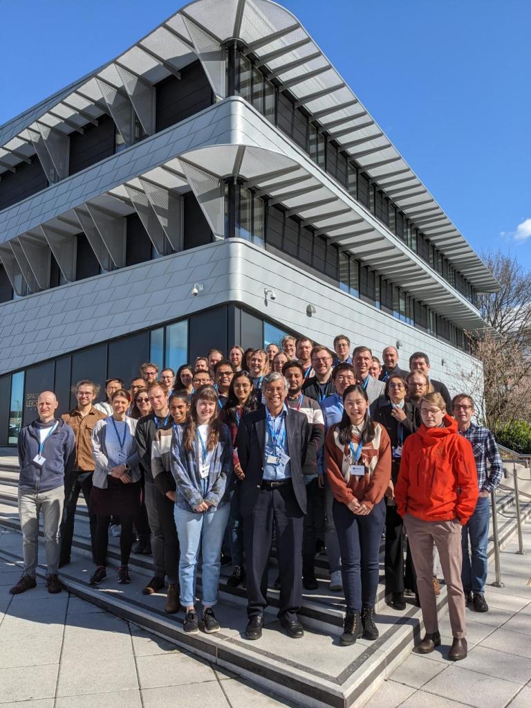
Every year, the Met PhD students at the University of Reading invite a scientist from a different university to learn from and talk to about their own project. This year we had the renowned Professor Tim Woolings, who currently researches and teaches at the University of Oxford. Tim’s interests generally revolve around large scale atmospheric dynamics and understanding the impacts of climate change on such features. We, as Met PhD students, were very excited and extremely thankful that Tim donated a week of his time (4th-8th of October) and travelled from Oxford for hybrid events within the Met. building. Tim told us of his own excitement to be back visiting Reading, after completing his PhD here, on isentropic modelling of the atmosphere, and staying on as a researcher and part of the department until 2013.
The week started with Tim presenting “Jet Stream Trends” at the Dynamical Research Group, known as Hoskin’s Half Hour. A large number of PhD students, post-doctorates and supervisors attended, which was to be expected considering Tim has a book dedicated on Jet streams. After a quick turnaround, he spoke at the departmental lunch time seminar on “The role of Rossby waves in polar weather and climate”. Here, Tim did an initial review on Rossby wave theory and then talked about his current fascinating research on the relevance of them within the polar atmosphere. The rest of Tim’s Monday consisted of lunch at park house with Robert Lee and the organising committee, Charlie Suitters, Hannah Croad and Isabel Smith (within picture). Later that evening Tim visited the Three Tuns pub with other staff members, for an important staff meeting! The PhD networking social with Tim on Thursday was a great evening where 15 to–20 students were able to discuss Tim’s research in a less formal setting within Park House pub.
Tim Woolings (2nd left) and the visiting scientist organising committee
Tim’s Tuesday, Wednesday (morning) and Thursday consisted of virtual and in-person one on one 15-minute meetings with PhD students. Here students explained their research projects and Tim gave them a refreshing outsider perceptive. On Wednesday afternoon, after Tim attended the High-Resolution Climate Modelling research group, he talked about his career in PhD group (A research group for PhD students only, where PhD students present to each other.). Tim explained how his PhD did not work as well as he had initially hoped, and the entire room felt a great weight of relief. His advice on keeping calm and looking for the bigger picture was heard by us all.
On Friday the 8th, a mini conference was put on and six students got to the “virtual” and literal stage and presented their current findings. Topics ranged from changes to Arctic cyclones, blocking, radar and Atmospheric dust. The conference and the week itself were both great successes, with PhD students leaving with inspiring questions to help aid their current studies. All at the University of Reading Department of Meteorology were extremely grateful and we thoroughly enjoyed having Tim here. We wish him all the best in his future endeavours and hope he comes back soon!


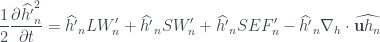
 is vertically-integrated FMSE,
  and
and  are the net atmospheric column longwave and shortwave heating rates,
  is the surface enthalpy flux, made up of the surface latent and sensible heat fluxes, and
  is the horizontal divergence of the
  ) indicate local anomalies from the instantaneous domain mean. The subscript (
 ) denotes a normalised variable which is the original variable divided by the difference between the hypothetical upper and lower limits of
  variance (left hand side term) is driven by interactions between
  anomalies and anomalies in normalised net longwave heating, shortwave heating, surface fluxes and advection.


 and
and  . We can see
  are closely correlated since
 and
and  and the Mature phase has
  and
and  . The contribution of longwave interactions with each cloud type to aggregation during these two phases is shown in Figure 5a, with their mean
  covariance and fraction shown in Figures 5b & c.

