The workshop was organised under the umbrella of ECMWF, the Copernicus services CEMS and C3S, the Hydrological Ensemble Prediction EXperiment (HEPEX) and the Global Flood Partnership (GFP). The workshop lasted 3 days, with a keynote speaker followed by Q&A at the start of each of the 6 sessions. Each keynote talk focused on a different part of the forecast chain, from hybrid hydrological forecasting to the use of forecasts for anticipatory humanitarian action, and how the global and local hydrological scales could be linked. Following this were speedy poster pitches from around the world and poster presentations and discussion in the virtual ECMWF (Gather.town).
Figure 1: Gather.town was used for the poster sessions and was set up to look like the ECMWF site in Reading, complete with a Weather Room and rubber ducks.
What was your poster about?
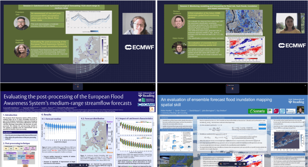
Gwyneth – I presented Evaluating the post-processing of the European Flood Awareness System’s medium-range streamflow forecasts in Session 2 – Catchment-scale hydrometeorological forecasting: from short-range to medium-range. My poster showed the results of the recent evaluation of the post-processing method used in the European Flood Awareness System. Post-processing is used to correct errors and account for uncertainties in the forecasts and is a vital component of a flood forecasting system. By comparing the post-processed forecasts with observations, I was able to identify where the forecasts were most improved.
Helen – I presented An evaluation of ensemble forecast flood map spatial skill in Session 3 – Monitoring, modelling and forecasting for flood risk, flash floods, inundation and impact assessments. The ensemble approach to forecasting flooding extent and depth is ideal due to the highly uncertain nature of extreme flooding events. The flood maps are linked directly to probabilistic population impacts to enable timely, targeted release of funding. The Flood Foresight System forecast flood inundation maps are evaluated by comparison with satellite based SAR-derived flood maps so that the spatial skill of the ensemble can be determined.
Figure 2: Gwyneth (left) and Helen (right) presenting their posters shown below in the 2-minute pitches.
What did you find most interesting at the workshop?
Gwyneth – All the posters! Every session had a wide range of topics being presented and I really enjoyed talking to people about their work. The keynote talks at the beginning of each session were really interesting and thought-provoking. I especially liked the talk by Dr Wendy Parker about a fitness-for-purpose approach to evaluation which incorporates how the forecasts are used and who is using the forecast into the evaluation.
Helen – Lots! All of the keynote talks were excellent and inspiring. The latest developments in detecting flooding from satellites include processing the data using machine learning algorithms directly onboard, before beaming the flood map back to earth! If openly available and accessible (this came up quite a bit) this will potentially rapidly decrease the time it takes for flood maps to reach both flood risk managers dealing with the incident and for use in improving flood forecasting models.
How was your virtual poster presentation/discussion session?
Gwyneth – It was nerve-racking to give the mini-pitch to +200 people, but the poster session in Gather.town was great! The questions and comments I got were helpful, but it was nice to have conversations on non-research-based topics and to meet some of the EC-HEPEXers (early career members of the Hydrological Ensemble Prediction Experiment). The sessions felt more natural than a lot of the virtual conferences I have been to.
Helen – I really enjoyed choosing my hairdo and outfit for my mini self. I’ve not actually experienced a ‘real’ conference/workshop but compared to other virtual events this felt quite realistic. I really enjoyed the Gather.town setting, especially the duck pond (although the ducks couldn’t swim or quack! J). It was great to have the chance talk about my work and meet a few people, some thought-provoking questions are always useful.
The focus of my PhD project is investigating the physical mechanisms behind the growth and evolution of summer-time Arctic cyclones, including the interaction between cyclones and sea ice. The rapid decline of Arctic sea ice extent is allowing human activity (e.g. shipping) to expand into the summer-time Arctic, where it will be exposed to the risks of Arctic weather. Arctic cyclones produce some of the most impactful Arctic weather, associated with strong winds and atmospheric forcings that have large impacts on the sea ice. Hence, there is a demand for improved forecasts, which can be achieved through a better understanding of Arctic cyclone mechanisms.
My PhD project is closely linked with a NERC project (Arctic Summer-time Cyclones: Dynamics and Sea-ice Interaction), with an associated field campaign. Whereas my PhD project is focused on Arctic cyclone mechanisms, the primary aims of the NERC project are to understand the influence of sea ice conditions on summer-time Arctic cyclone development, and the interaction of cyclones with the summer-time Arctic environment. The field campaign, originally planned for August 2021 based in Svalbard in the Norwegian Arctic, has now been postponed to August 2022 (due to ongoing restrictions on international travel and associated risks for research operations due to the evolving Covid pandemic). The field campaign will use the British Antarctic Survey’s low-flying Twin Otter aircraft, equipped with infrared and lidar instruments, to take measurements of near-surface fluxes of momentum, heat and moisture associated with cyclones over sea ice and the neighbouring ocean. These simultaneous observations of turbulent fluxes in the atmospheric boundary layer and sea ice characteristics, in the vicinity of Arctic cyclones, are needed to improve the representation of turbulent exchange over sea ice in numerical weather prediction models.
Those wishing to fly onboard the Twin Otter research aircraft are required to do Helicopter Underwater Escape Training (HUET). Most of the participants on the course travel to and from offshore facilities, as the course is compulsory for all passengers on the helicopters to rigs. In the unlikely event that a helicopter must ditch on the ocean, although the aircraft has buoyancy aids, capsize is likely because the engine and rotors make the aircraft top heavy. I was apprehensive about doing the training, as having to escape from a submerged aircraft is not exactly my idea of fun. However, I realise that being able to fly on the research aircraft in the Arctic is a unique opportunity, so I was willing to take on the challenge!
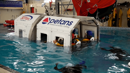
The HUET course is provided by the Petans training facility in Norwich. John Methven, Ben Harvey, and I drove to Norwich the night before, in preparation for an early start the next day. We spent the morning in the classroom, covering helicopter escape procedures and what we should expect for the practical session in the afternoon. We would have to escape from a simulator recreating a crash landing on water. The simulator replicates a helicopter fuselage, with seats and windows, attached to the end of a mechanical arm for controlled submersion and rotation. The procedure is (i) prepare for emergency landing: check seatbelt is pulled tight, headgear is on, and that all loose objects are tucked away, (ii) assume the brace position on impact, and (iii) keep one hand on the window exit and the other on your seatbelt buckle. Once submerged, undo your seatbelt and escape through the window. After a nervy lunch, it was time to put this into practice.
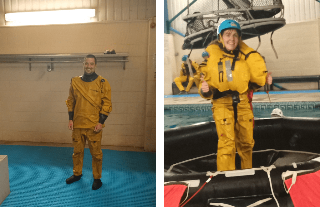
The practical part of the course took place in a pool (the temperature resembled lukewarm bath water, much warmer than the North Atlantic!). We were kitted up with two sets of overalls over our swimming costumes, shoes, helmets, and jackets containing a buoyancy aid. We then began the training in the aircraft simulator. Climb into the aircraft and strap yourself into a seat. The seatbelt had to be pulled tight, and was released by rotating the central buckle. On the pilots command, prepare for emergency landing. Assume the brace position, and the aircraft drops into the water. Hold on to the window and your seatbelt buckle, and as the water reaches your chest, take a deep breath. Wait for the cabin to completely fill with water and stop moving – only then undo your seatbelt and get out!
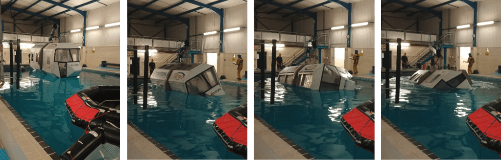
The practical session consisted of three parts. In the first exercise, the aircraft was submerged, and you had to escape through the window. The second exercise was similar, except that panes were fitted on the windows, which you had to push out before escaping. In the final exercise, the aircraft was submerged and rotated 180 degrees, so you ended up upside down (and with plenty of water up your nose), which was very disorientating! Each exercise required you to hold your breath for roughly 10 seconds at a time. Once we had escaped and reached the surface, we deployed our buoyancy aids, and climbed to safety onto the life raft.
Going for a spin! The aircraft simulator being rotated with me strapped in
Ben and I happy to have survived the training!
The experience was nerve-wracking, and really forced me to push myself out of my comfort zone. I didn’t need to be too worried though, even after struggling with undoing the seatbelt a couple of times, I was assisted by the diving team and encouraged to go again. I was glad to get through the exercises, and pass the course along with the others. This was an amazing experience (definitely not something I expected to do when applying for a PhD!), and I’m now looking forward to the field campaign next year.
A week-long summer school on forecast verification was held jointly at the end of June by the MPECDT (Mathematics of Planet Earth Centre for Doctoral Training) and JWGFVR (Joint Working Group on Forecast Verification Research). The school featured lectures from scientists and academics from many different countries around the world including Brazil, USA and Canada. They each specialised in different topics within forecast verification. Participants gained a large overview of the field and how the fields within it interact.
Structure of school
The virtual school consisted of lectures from individual members of the JWGFVR on their own subjects, along with drop-in sessions for asking questions and dedicated time to work on group projects. Four groups of 4-5 students were given an individual forecast verification challenge. The themes of the projects were precipitation forecasts, comparing high resolution global model and local area model wind speed forecasts, and ensemble seasonal forecasts. The latter was the topic of our project.
Content
The first lecture was given by Barbara Brown, who provided a broad summary of verification and gave examples of questions that verifiers may ask themselves as they attempt to assess the “goodness” of a forecast. The next day, a lecture by Barbara Casati covered continuous scores (verification of continuous variables e.g., temperature), such as linear bias, mean-squared error (MSE) and Pearson coefficient. She also outlined the deficits of different scores and how it is best to use a variety of them when assessing the quality of a forecast. Marion Mittermaier then spoke about categorical scores (yes/no events or multi category events such as precipitation type). She gave examples such as contingency tables which portray how well a model is able to predict a given event, based on hit rates (how often the model predicted an event when the event happened), and false alarm rates (how often the model predicted the event when it didn’t happen). Further lectures were given by Ian Joliffe on methods of determining the significance of your forecast scores, Nachiketa Acharya on probabilistic scores and ensembles, Caio Coelho on sub-seasonal to seasonal timescales, and then Raghavendra Ashrit, Eric Gilleland and Caren Marzban on severe weather, spatial verification and experimental design. The lectures have been made available online and you can find them here.
Forecast Verification
So, forecast verification is as it sounds: a part of assessing the ‘goodness’ of a forecast as opposed to its value. Verification is helpful for economic purposes (e.g. decision making), as well as administrative and scientific ones (e.g. identifying model flaws). The other aspect of measuring how well a forecast is performing is knowing the user’s needs, and therefore how to apply the forecast. It is important to consider the goal of your verification process beforehand, as it will outline your choice of metrics and your assessment of them. An example of how forecast goodness hinges on the user was given by Barbara in her talk: a precipitation forecast may have a spatial offset of where a rain patch falls, but if both observation and forecast fall along the flight path, this may be all the aviation traffic strategic planner needs to know. For a watershed manager on the ground, however, this would not be a helpful forecast. The lecturers also emphasised the importance of performing many different measures on a forecast and then understanding the significance of your measures in order to help you understand its overall goodness. Identifying standards of comparison for your forecast is also important, such as persistence or climatology. Then there are further challenges such as spatial verification, which requires methods of ‘matching’ the location of your observations with the model predictions on the model grid.
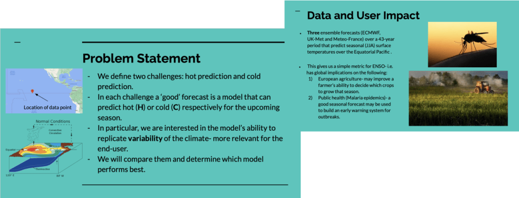
Figure 1: Problem statement for group presentation on 2m temperature ensemble seasonal forecasts, presented by Ryo Kurashina
Group Project
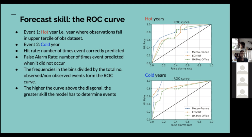
Our project was on verification of 2 metre temperature ensemble seasonal forecasts (see Figure 1). We were looking at seasonal forecast data with a 1-month lead time for the summer months for three different models and investigating ways of validating the forecasts, finally deciding which one was the better. We decided to focus on the models’ ability to predict hot and cold events as a simple metric for El Nino. We looked at scatter plots and rank histograms to investigate the biases in our data, Brier scores for assessing model accuracy (level of agreement between forecast and truth) and Receiver Operating Characteristic curves to look model skill (the relative accuracy of the forecast over some reference forecast). The ROC curve (see Fig. 2) refers to the curve formed by plotting hit rates against false alarm rates based on probability thresholds. The further above the diagonal line your curve lies, the better your forecast is at discriminating events compared to a random coin toss. The combination of these verification methods were used to assess which model we thought was best.
Of course, virtual summer schools are less than ideal compared to the real (in person) deal, but with Teams meetings, shared code and chat channel we made the most of it. It was fun to work with everyone, even (or especially?) if the topic was new for all of us.
Figure 2: Presenting our project during group project presentations on Friday
Conclusions
The summer school was incredibly smoothly run, very engaging to people both new and experienced in the topic and provided plenty of opportunity to ask questions to the enthusiastic lecturers. Would recommend to PhD students working with forecasts and wanting to assess them!
Andrea Marcheggiani – a.marcheggiani@pgr.reading.ac.uk
Diabatic processes are typically considered as a source of energy for weather systems and as a primary contributing factor to the maintenance of mid-latitude storm tracks (see Hoskins and Valdes 1990 for some classical reading, but also a more recent reviews, e.g. Chang et al. 2002). However, surface heat exchanges do not necessarily act as a fuel for the evolution of weather systems: the effects of surface heat fluxes and their coupling with lower-tropospheric flow can be detrimental to the potential energy available for systems to grow. Indeed, the magnitude and sign of their effects depend on the different time (e.g., synoptic, seasonal) and length (e.g., global, zonal, local) scales which these effects unfold at.
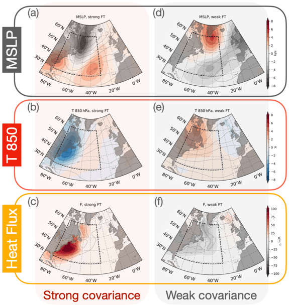
Figure 1: Composites for strong (a-c) and weak (d-f) values of the covariance between heat flux and temperature time anomalies.
Heat fluxes arise in response to thermal imbalances which they attempt to neutralise. In the atmosphere, the primary thermal imbalances that are observed correspond with the meridional temperature gradient caused by the equator—poles differential radiative heating from the Sun, and the temperature contrasts at the air—sea interface which essentially derives from the different heat capacities of the oceans and the atmosphere.
In the context of the energetic scheme of the atmosphere, which was first formulated by Lorenz (1955) and commonly known as Lorenz energy cycle, the meridional transport of heat (or dry static energy) is associated with conversion of zonal available potential energy to eddy available potential energy, while diabatic processes at the surface coincide with generation of eddy available potential energy.
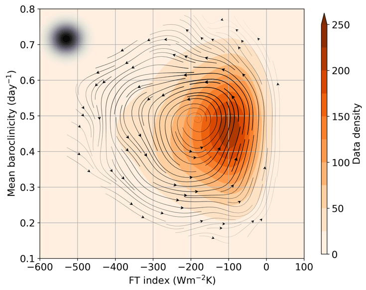
Figure 2: Phase portrait of FT covariance and mean baroclinicity. Streamlines indicate average circulation in the phase space (line thickness proportional to phase speed). The black shaded dot in the top left corner indicates the size of the Gaussian kernel used in the smoothing process. Colour shading indicates the number of data points contributing to the kernel average
The sign of the contribution from surface heat exchanges to the evolution on weather systems is not univocal, as it depends on the specific framework which is used to evaluate their effects. Globally, these have been estimated to have a positive effect on the potential energy budget (Peixoto and Oort, 1992) while locally the picture is less clear, as heating where it is cold and cooling where it is warm would lead to a reduction in temperature variance, which is essentially available potential energy.
The first part of my PhD focussed on assessing the role of local air—sea heat exchanges on the evolution of synoptic systems. To that extent, we built a hybrid framework where the spatial covariance between time anomalies of sensible heat flux F and lower-tropospheric air temperature T is taken as a measure of the intensity of the air—sea thermal coupling. The time anomalies, denoted by a prime, are defined as departures from a 10-day running mean so that we can concentrate on synoptic variability (Athanasiadis and Ambaum, 2009). The spatial domain where we compute the spatial covariance extends from 30°N to 60°N and from 30°W to 79.5°W, which corresponds with the Gulf Stream extension region, and to focus on air—sea interaction, we excluded grid points covered by land or ice.
This leaves us with a time series for F’—T’ spatial covariance, which we also refer to as FT index.
The FT index is found to be always positive and characterised by frequent bursts of intense activity (or peaks). Composite analysis, shown in Figure 1 for mean sea level pressure (a,d), temperature at 850hPa (b,e) and surface sensible heat flux (c,f), indicates that peaks of the FT index (panels a—c) correspond with intense weather activity in the spatial domain considered (dashed box in Figure 1) while a more settled weather pattern is observed to be typical when the FT index is weak (panels d—f).
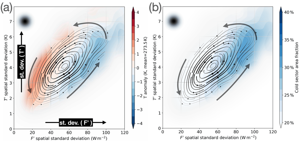
Figure 3: Phase portraits for spatial-mean T (a) and cold sector area fraction (b). Shading in (a) represents the difference between phase tendency and the mean value of T, as reported next to the colour bar. Arrows highlight the direction of the circulation, kernel-averaged using the Gaussian kernel shown in the top-left corner of each panel.
We examine the dynamical relationship between the FT index and the area-mean baroclinicity, which is a measure of available potential energy in the spatial domain. To do that, we construct a phase space of FT index and baroclinicity and study the average circulation traced by the time series for the two dynamical variables. The resulting phase portrait is shown in Figure 2. For technical details on phase space analysis refer to Novak et al. (2017), while for more examples of its use see Marcheggiani and Ambaum (2020) or Yano et al. (2020). We observe that, on average, baroclinicity is strongly depleted during events of strong F’—T’ covariance and it recovers primarily when covariance is weak. This points to the idea that events of strong thermal coupling between the surface and the lower troposphere are on average associated with a reduction in baroclinicity, thus acting as a sink of energy in the evolution of storms and, more generally, storm tracks.
Upon investigation of the driving mechanisms that lead to a strong F’—T’ spatial covariance, we find that increases in variances and correlation are equally important and that appears to be a more general feature of heat fluxes in the atmosphere, as more recent results appear to indicate (which is the focus of the second part of my PhD).
In the case of surface heat fluxes, cold sector dynamics play a fundamental role in driving the increase of correlation: when cold air is advected over the ocean surface, flux variance amplifies in response to the stark temperature contrasts at the air—sea interface as the ocean surface temperature field features a higher degree of spatial variability linked to the presence of both the Gulf Stream on the large scale and oceanic eddies on the mesoscale (up to 100 km).
The growing relative importance of the cold sector in the intensification phase of the F’—T’ spatial covariance can also be revealed by looking at the phase portraits for air temperature and cold sector area fraction, which is shown in Figure 3. These phase portraits tell us how these fields vary at different points in the phase space of surface heat flux and air temperature spatial standard deviations (which correspond to the horizontal and vertical axes, respectively). Lower temperatures and larger cold sector area fraction characterise the increase in covariance, while the opposite trend is observed in the decaying stage.
Surface heat fluxes eventually trigger an increase in temperature variance, which within the atmospheric boundary layer follows an almost adiabatic vertical profile which is characteristic of the mixed layer (Stull, 2012).
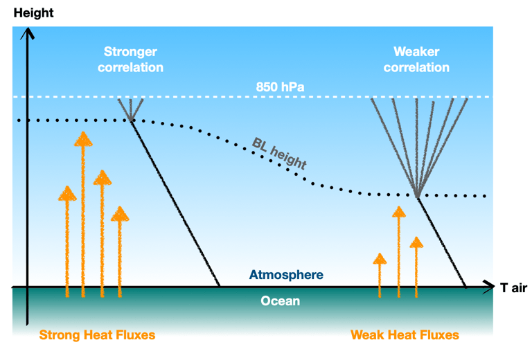
Figure 4: Diagram of the effect of the atmospheric boundary layer height on modulating surface heat flux—temperature correlation.
Stronger surface heat fluxes are associated with a deeper boundary layer reaching higher levels into the troposphere: this could explain the observed increase in correlation as the lower-tropospheric air temperatures become more strongly coupled with the surface, while a lower correlation with the surface ensues when the boundary layer is shallow and surface heat flux are weak. Figure 4 shows a simple diagram summarising the mechanisms described above.
In conclusion, we showed that surface heat fluxes locally can have a damping effect on the evolution of mid-latitude weather systems, as the covariation of surface heat flux and air temperature in the lower troposphere corresponds with a decrease in the available potential energy.
Results indicate that most of this thermodynamically active heat exchange is realised within the cold sector of weather systems, specifically as the atmospheric boundary layer deepens and exerts a deeper influence upon the tropospheric circulation.
References
Athanasiadis, P. J. and Ambaum, M. H. P.: Linear Contributions of Different Time Scales to Teleconnectivity, J. Climate, 22, 3720– 3728, 2009.
Chang, E. K., Lee, S., and Swanson, K. L.: Storm track dynamics, J. Climate, 15, 2163–2183, 2002.
Hoskins, B. J. and Valdes, P. J.: On the existence of storm-tracks, J. Atmos. Sci., 47, 1854–1864, 1990.
Lorenz, E. N.: Available potential energy and the maintenance of the general circulation, Tellus, 7, 157–167, 1955.
Marcheggiani, A. and Ambaum, M. H. P.: The role of heat-flux–temperature covariance in the evolution of weather systems, Weather and Climate Dynamics, 1, 701–713, 2020.
Novak, L., Ambaum, M. H. P., and Tailleux, R.: Marginal stability and predator–prey behaviour within storm tracks, Q. J. Roy. Meteorol. Soc., 143, 1421–1433, 2017.
Peixoto, J. P. and Oort, A. H.: Physics of climate, American Institute of Physics, New York, NY, USA, 1992.
Stull, R. B.: Mean boundary layer characteristics, In: An Introduction to Boundary Layer Meteorology, Springer, Dordrecht, Germany, 1–27, 1988.
Yano, J., Ambaum, M. H. P., Dacre, H., and Manzato, A.: A dynamical—system description of precipitation over the tropics and the midlatitudes, Tellus A: Dynamic Meteorology and Oceanography, 72, 1–17, 2020.