Sting Jet: the poisonous (and windy) tail of some of the most intense UK storms

Email: a.volonte@pgr.reading.ac.uk

IDL TIFF file
Figure 1: Windstorm Tini (12 Feb 2014) passes over the British Isles bringing extreme winds. A Sting Jet has been identified in the storm. Image courtesy of NASA Earth Observatory

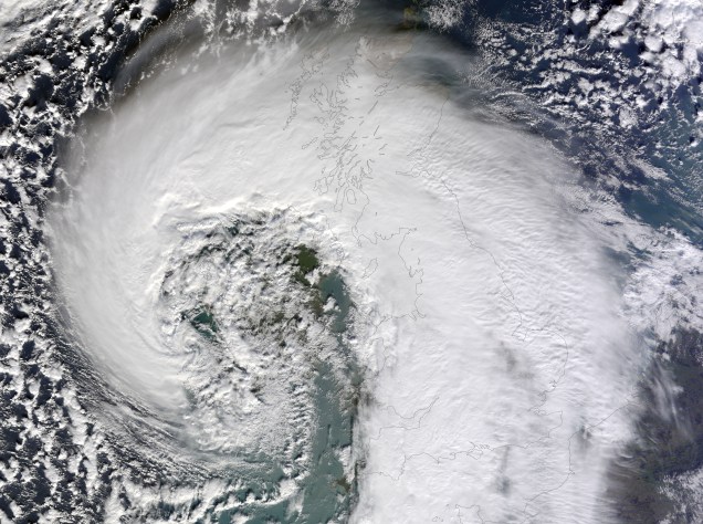
It was the morning of 16th October when South East England got battered by the Great Storm of 1987. Extreme winds occurred, with gusts of 70 knots or more recorded continually for three or four consecutive hours and maximum gusts up to 100 knots. The damage was huge across the country with 15 million trees blown down and 18 fatalities.

case_study_great_storm_fig011
Figure 2: Surface wind gusts in the Great Storm of 1987. Image courtesy of UK Met Office.

The forecast issued on the evening of 15th October failed to identify the incoming hazard but forecasters were not to blame as the strongest winds were actually due to a phenomenon that had yet to be discovered at the time: the Sting Jet. A new topic of weather-related research had started: what was the cause of the exceptionally strong winds in the Great Storm?

It was in Reading at the beginning of 21st century that scientists came up with the first formal description of those winds, using observations and model simulations. Following the intuitions of Norwegian forecasters they used the term Sting Jet, the ‘sting at the end of the tail’. Using some imagination we can see the resemblance of the bent-back cloud head with a scorpion’s tail: strong winds coming out from its tip and descending towards the surface can then be seen as the poisonous sting at the end of the tail.

Conceptual+model+of+storm+development
Figure 3: Conceptual model of a sting-jet extratropical cyclone, from Clark et al, 2005. As the cloud head bends back and the cold front moves ahead we can see the Sting Jet exiting from the cloud tip and descending into the opening frontal fracture.  WJ: Warm conveyor belt. CJ: Cold conveyor belt. SJ: Sting jet.

In the last decade sting-jet research progressed steadily with observational, modelling and climatological studies confirming that the strong winds can occur relatively often, that they form in intense extratropical cyclones with a particular shape and are caused by an additional airstream that is neither related to the Cold nor to the Warm Conveyor Belt. The key questions are currently focused on the dynamics of Sting Jets: how do they form and accelerate?

Works recently published (and others about to come out, stay tuned!) claim that although the Sting Jet occurs in an area in which fairly strong winds would already be expected given the morphology of the storm, a further mechanism of acceleration is needed to take into account its full strength. In fact, it is the onset of mesoscale instabilities and the occurrence of evaporative cooling on the airstream that enhances its descent and acceleration, generating a focused intense jet (see references for more details). It is thus necessary a synergy between the general dynamics of the storm and the local processes in the cloud head in order to produce what we call the Sting Jet .

plot_3D_sj ccb_short
Figure 4: Sting Jet (green) and Cold Conveyor Belt (blue) in the simulations of Windstorm Tini. The animation shows how the onset of the strongest winds is related to the descent of the Sting Jet. For further details on this animation and on the analysis of Windstorm Tini see here.

References:

http://www.metoffice.gov.uk/learning/learn-about-the-weather/weather-phenomena/case-studies/great-storm

Browning, K. A. (2004), The sting at the end of the tail: Damaging winds associated with extratropical cyclones. Q.J.R. Meteorol. Soc., 130: 375–399. doi:10.1256/qj.02.143

Clark, P. A., K. A. Browning, and C. Wang (2005), The sting at the end of the tail: Model diagnostics of fine-scale three-dimensional structure of the cloud head. Q.J.R. Meteorol. Soc., 131: 2263–2292. doi:10.1256/qj.04.36

Martínez-Alvarado, O., L.H. Baker, S.L. Gray, J. Methven, and R.S. Plant (2014), Distinguishing the Cold Conveyor Belt and Sting Jet Airstreams in an Intense Extratropical Cyclone. Mon. Wea. Rev., 142, 2571–2595, doi: 10.1175/MWR-D-13-00348.1.

Hart, N.G., S.L. Gray, and P.A. Clark, 0: Sting-jet windstorms over the North Atlantic: Climatology and contribution to extreme wind risk. J. Climate, 0, doi: 10.1175/JCLI-D-16-0791.1.

Volonté, A., P.A. Clark, S.L. Gray. The role of Mesoscale Instabilities in the Sting-Jet dynamics in Windstorm Tini. Poster presented at European Geosciences Union – General Assembly 2017, Dynamical Meteorology (General session)

Prof. Tapio Schneider – Our Distinguished PhD Visiting Scientist.

Email: j.f.talib@pgr.reading.ac.uk

Every year PhD students from the Department of Meteorology at the University of Reading welcome a distinguished scientist in the field of environmental sciences. Previous scientists include Richard Rotunno (UCAR), Isaac Held (GFDL) and Susan Solomon (NOAA). This year’s honoured visitor was Professor Tapio Schneider from the climate dynamics research group from California Institute of Technology (Caltech), the academic home of NASA’s Jet Propulsion Laboratory. Tapio is a well-known contributor to our understanding of global climate dynamics and it was a pleasure to welcome him to our department.

SAMSUNG CSC
Prof. Tapio Schneider with some of the current PhD cohort.

Our visiting scientist programme in the department is an opportunity for PhD students to share and explain their research to an external visitor. It allows for PhD research to be looked at from a completely new perspective which will hopefully improve the PhD studies. In a typical PhD visiting scientist week, the visiting scientist meets students one to one, attends departmental research groups and presents work in departmental seminars.

Tapio Schneider presented two departmental seminars during his time with us titled How low clouds respond to warming: Observational, numerical and physical constraints and Model hierachies: From advancing climate dynamics to improving predictions. The latter of these seminars encouraged a discussion to rethink how we approach advancing our modelling capabilities. Tapio argued that the atmospheric modelling community had not fully engaged in the benefits that observations offer. He suggested that our goal should be a heirarchical system that integrates both observational data and models. We should look into creating “machine-learning” models, those which use observational data to improve our modelling capabilities through altering parameterisation schemes and radiative balance calculations at the top of the atmosphere (as two examples).

As already mentioned, the visiting scientist also meets with students one-to-one and it was highly beneficial for my own project to have a meeting with Tapio Schneider. We discussed papers released by himself alongside his former PhD student Tobias Bischoff (for example, The Equatorial Energy Balance, ITCZ position and Double-ITCZ bifurications) which concentrate on creating a diagnostic framework with which we can estimate the location and structure of the Inter-Tropical Convergence Zone (ITCZ). We discussed conclusions reached from my own aquaplanet simulations and how they relate to the proposed diagnostic framework. Keep an eye on the blog for a post coming soon on the developments in my own PhD project, (titled, what determines the location and intensity of the ITCZ?).

To bring this blog post to a close I would like to thank Professor Tapio Schneider for his time, knowledge and wisdom that he shared with the PhD cohort whilst at Reading. Thank you also to those from the University of Reading who supported Tapio’s visit. Feedback from the PhD cohort is extremely positive and I would highly recommend a similar scheme for other scientific departments.

20170508_193056
PhD social with the distinguished visitor.

Under-ice melt ponds in the Arctic

Email: n.e.smith@pgr.reading.ac.uk

The Arctic’s climate is one of those most rapidly changing globally, and as such the region has become a poster-child of climate change. Sea ice area is frequently used as an indicator of the rate of change of the system, providing striking visualisations of the rapidity of the change in recent years. The sea ice is also a driver of climate change, with areal cover greatly affecting the planet’s albedo and ice melt cooling and desalinating the Arctic ocean, altering circulation globally.

meltwaterLayerHHopNorskPolarinstitutt

Photo: Haakon Hop, Norsk Polarinstitutt

During the summer months, incoming solar radiation melts the surface layers of the sea ice. This melt water collects in hollows on the surface of the sea ice forming pools called melt ponds. Since the sea ice is porous, water from these ponds can percolate down or flow down through macroscopic flaws in the ice and out of the base of the ice. The melt water is relatively warm and fresh compared to the ocean below, so it floats between the ice and the ocean, gathering in pools beneath the sea ice called under-ice melt ponds. [1]

A couple of types of ice growth have been observed associated with these ponds. Most importantly, a sheet of ice can form at the interface between the pond and the ocean, completely isolating the fresh water from the ocean. As they create the illusion that they are the base of the sea ice, these sheets of ice are commonly referred to as ‘false bottoms’. [2]

We have developed a one-dimensional thermodynamic model of under-ice melt ponds to investigate how they affect their surroundings. We have carried out a number of sensitivity studies using this model, which have lead to some interesting conclusions about how these ponds evolve and affect the ice above them.

For example, the thicker the sea ice above an under-ice melt pond, the longer it takes to freeze due to a shallower temperature gradient above. As a result, more ice is gained due to under-ice melt ponds beneath thicker ice. This could be a positive feedback cycle, since we expect to see thinner ice on average as the Arctic warms, leading to less ice gained due to the ponds beneath it.

eguSens0

We also see that, as well as the outcome observed in the field, in which the false bottom migrates upwards and thickens as it freezes through the pond, it can also ablate under certain conditions. For example, ponds that are relatively salty at the start of the simulation freeze more slowly, and the false bottom ablates before it is able to reach the base of the sea ice.

eguSens1

Our sensitivity studies show that under-ice melt ponds could be responsible for up to 7.9% additional ice thickness at the end of a 50 day simulation. This would equate to up to 3.2% more ice volume across the Arctic dependent on the area of the ice underlain by these pools.

Recently, we have coupled our under-ice melt pond model with a simple, zero-dimensional model of the oceanic mixed layer. Using this coupled model, we see that the false bottom ablates more rapidly than a slab of sea ice, releasing more fresh water into the mixed layer. This strong reduction of salinity causes a shallowing of the mixed layer. We are currently further investigating the effects that the ponds have on the ocean below them.

Under-ice melt ponds and false bottom insulate the sea ice from below and affect the basal fluxes of salt and fresh water into the mixed layer, and thicken the ice above them allowing less radiation to penetrate through from the surface. They are clearly significant to the mass balance of the ice and the ocean below them, yet are not currently accounted for in the sea ice components of climate models. A parameterisation of their effects would be useful to include.

[1] Notz, Dirk, et al. “Impact of underwater‐ice evolution on Arctic summer sea ice.” Journal of Geophysical Research: Oceans 108.C7 (2003).

[2] Martin, Seelye, and Peter Kauffman. “The evolution of under-ice melt ponds, or double diffusion at the freezing point.” Journal of Fluid Mechanics 64.3 (1974): 507-528.

A PhD Student’s Guide to EGU 2017

Email: r.frew@pgr.reading.ac.uk

EGU2017logo

Science is a community effort, requiring collaboration and lots of different people providing different parts of the jigsaw to try to understand more and more of the full picture. Despite a lot of research being carried out individually in a lab, or at a desk, no one individual can do everything themselves, no matter how much of a genius they are. Sharing, discussing and debating are key to the progression of scientific ideas, and this ethos is something large scientific conferences like EGU cultivates.

Attending EGU for the first time as a PhD student was both an exciting and overwhelming experience due to its shear size and number of people. This year 14,496 people from 107 countries participated, giving 4,849 talks, 11,312 posters and 1,238 PICO presentations throughout the week!  

With 649 scientific sessions running throughout the week, deciding how to spend your day was a significant challenge in itself! The EGU website and app allowed you to create a personal programme, cutting down the number of entire printed programmes being printed, aiming to try to make EGU slightly more environmentally friendly.

IMG_2541
Vienna international conference centre, image courtesy of Matt Priestley.

A ‘typical’ day at EGU consisted of something like… 

7-8am: Wake up, shower and breakfast and then hop on the U-bahn to the conference centre. Pick up a EGU Today newsletter on the way into the centre, highlighting a few sessions happening that day that may be of general interest

8.30-10am: Division session of your choice consisting of six 15min talks. People also pick out specific talks in different sessions and hop between, especially if their work is more interdisciplinary and covers a few different sessions.

10-10.30am: Recharge with a much needed coffee break!

10.30am-12pm: Go to a debate on ‘Make Facts Great Again: how can scientists stand up for science?‘ There were a number of other topical debates throughout the week, including ‘Arctic environmental change: global opportunities and threats‘ and ‘Great Debate on Great Extinctions‘. This consisted of a short introduction from members of a panel, then questions from the floor.

12-1.30pm: Pick up something for lunch from one of the nearby bakeries or cafes around the conference centre, and sit in the nearby park and enjoy the sunshine (hopefully).

1.30-3pm: Explore the many information stands in the exhibition areas. These included publishing houses, geoscience companies, NGOs etc. Next go and vote in the EGU photograph competition: https://imaggeo.egu.eu/photo-contest/2017/, before stopping to listen to some PICO (Presenting Interactive COntent) presentations. These are very interactive sessions where speakers give a 2min overview of their work, after which people have the opportunity to go and question speakers further afterwards by a poster/couple of slides.

3-3.30pm: Tea/coffee break with cookies in the Early Career Scientists lounge.

3.30-5pm: Polar Science Career Session aimed at Early Career Scientists (there were also sessions for other divisions), consisting of an informal Q&A with a panel covering a variety of different career paths.

5-7pm: Poster sessions in the big halls with beer/juice and nibbles. These were a great opportunity for in depth discussion, and meeting other people in your field.

7-8.30pm: Early career scientist (ECS) reception with drinks and canapes, meet other ECS from all fields and chat with division leaders. This year 53% of EGU participants were ECSs, and there was a definite effort to cater for them throughout the week.

8.30-?: Dinner and drinks in Vienna town centre with peers, followed by an early night if you plan to make it to a 8.30am session tomorrow…

EGU2017photowinners
EGU 2017 photo competition entries, image taken from the GeoLog blog, more information about the entries and results can be found at: http://blogs.egu.eu/geolog/2017/04/28/at-the-assembly-2017-friday-highlights/

In addition to events highlighted, there were also a variety short courses running, for example ‘Tips and Tricks: How to Navigate EGU‘, ‘How to write a research grant‘ or ‘Rhyme your Research‘! EGU had its own official blog GeoLog, highlighting some of the events from each day: http://blogs.egu.eu/geolog/.

However, EGU is 5 days long, and despite the impressive offering of sessions being put on it would be a shame to go to Vienna and only see the conference centre… The odd extended lunch break to take the U-bahn (included as part of the entrance to the conference) to walk around the centre, or an afternoon off to explore a gallery or museum, or simply sit in one of the beautiful parks or cafes to enjoy some coffee and Sachertorte is definitely a must to recharge and finish off the week!