Modelling – Page 5 – The Social Metwork

Stationary Orographic Rainbands

December 8, 2016Carly Wright1 Comment

Email: c.j.wright@pgr.reading.ac.uk

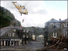
Small-scale rainbands often form downwind of mountainous terrain. Although relatively small in scale (a few tens of km across by up to ~100 km in length), these often poorly forecast bands can cause localised flooding as they can be associated with intense precipitation over several hours due to the anchoring effect of orography (Barrett et al., 2013). Figure 1 shows a flash flood caused by a rainband situated over Cockermouth in 2009. In some regions of southern France orographic banded convection can contribute 40% of the total rainfall (Cosma et al., 2002). Rainbands occur in various locations and under different synoptic regimes and environmental conditions making them difficult to examine their properties and determine their occurrence in a systematic way (Kirshbaum et al. 2007a,b, Fairman et al. 2016). My PhD considers the ability of current operational forecast models to represent these bands and the environmental controls on their formation.

blogfig1 — Figure 1: Flash flood event caused by a rainband situated over Cockermouth, Cumbria, UK in 2009

What is a rainband?

A cloud and precipitation structure associated with an area of rainfall which is significantly elongated
Stationary (situated over the same location) with continuous triggering
Can form in response to moist, unstable air following over complex terrain
Narrow in width ~2-10 km with varying length scales from 10 – 100’s km

blogfig2 — Figure 2: Schematic showing the difference between cellular and banded convection

To examine the ability of current operational forecast models to represent these bands a case study was chosen which was first introduced by Barrett, et al. (2016). The radar observations during the event showed a clear band along The Great Glen Fault, Scotland (Figure 3). However, Barrett, et al. (2016) concluded that neither the operational forecast or the operational ensemble forecast captured the nature of the rainband. For more information on ensemble models see one of our previous blog posts by David Flack Showers: How well can we predict them?.

blogfig3 — Figure 3: Radar observations of precipitation accumulation over a six hour period (between 3-9 am) showing a rainband located over The Great Glen Fault, Scotland on 29 December 2012.

Localised convergence and increased convective available potential energy along the fault supported the formation of the rainband. To determine the effect of model resolution on the model’s representation of the rainband, a forecast was performed with the horizontal gird spacing decreased to 500 m from 1.5 km. In this forecast a rainband formed in the correct location which generated precipitation accumulations close to those observed, but with a time displacement. The robustness of this forecast skill improvement is being assessed by performing an ensemble of these convection-permitting simulations. Results suggest that accurate representation of these mesoscale rainbands requires resolutions higher than those used operationally by national weather centres.

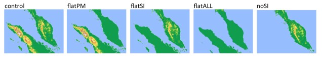
Idealised numerical simulations have been used to investigate the environmental conditions leading to the formation of these rainbands. The theoretical dependence of the partitioning of dry flow over and around mountains on the non-dimensional mountain height is well understood. For this project I examine the effect of this dependence on rainband formation in a moist environment. Preliminary analysis of the results show that the characteristics of rainbands are controlled by more than just the non-dimensional mountain height, even though this parameter is known to be sufficient to determine flow behaviour relative to mountains.

This work has been funded by the Natural Environmental Research Council (NERC) under the project PREcipitation STructures over Orography (PRESTO), for more project information click here.

References

Barrett, A. I., S. L. Gray, D. J. Kirshbaum, N. M. Roberts, D. M. Schultz, and J. G. Fairman, 2015: Synoptic Versus Orographic Control on Stationary Convective Banding. Quart. J. Roy. Meteorol. Soc., 141, 1101–1113, doi:10.1002/qj.2409.

— 2016: The Utility of Convection-Permitting Ensembles for the Prediction of Stationary Convective Bands. Mon. Wea. Rev., 144, 10931114, doi:10.1175/MWR-D-15-0148.1.

Cosma, S., E. Richard, and F. Minsicloux, 2002: The Role of Small-Scale Orographic Features in the Spatial Distribution of Precipitation. Quart. J. Roy. Meteorol. Soc., 128, 75–92, doi:10.1256/00359000260498798.

Fairman, J. G., D. M. Schultz, D. J. Kirshbaum, S. L. Gray, and A. I. Barrett, 2016: Climatology of Banded Precipitation over the Contiguous United States. Mon. Wea. Rev., 144,4553–4568, doi: 10.1175/MWR-D-16-0015.1.

Kirshbaum, D. J., G. H. Bryan, R. Rotunno, and D. R. Durran, 2007a: The Triggering of Orographic Rainbands by Small-Scale Topography. J. Atmos. Sci., 64, 1530–1549, doi:10.1175/JAS3924.1.

Kirshbaum, D. J., R. Rotunno, and G. H. Bryan, 2007b: The Spacing of Orographic Rainbands Triggered by Small-Scale Topography. J. Atmos. Sci., 64, 4222–4245, doi:10.1175/2007JAS2335.1.

Showers: How well can we predict them?

November 24, 2016David Flack1 Comment

Email: d.l.a.flack@pgr.reading.ac.uk

Showers are one of the many examples of convective events experienced in the UK, other such events include thunderstorms, supercells and squall lines. These type of events form most often in the summer but can also form over the sea in the winter. They form because the atmosphere is unstable, i.e. warm air over a cooler surface, this results in the creation of thermals. If there is enough water vapour in the air and the thermal reaches high enough the water vapour will condense and eventually form a convective cloud. Convective events produce intense, often very localised, rainfall, which can result in flash floods, e.g. Boscastle 2004.

boscastle04 — Boscastle flood 2004 – BBC News

Flash floods are very difficult to predict, unlike flood events that happen from the autumnal and winter storms e.g. floods from Storms Desmond and Frank last winter, and the current floods (20-22 November). So often there is limited lead time for emergency services to react to flash flood events. One of the main reasons why flash floods are difficult to predict is the association with convective events because these events only last for a few hours (6 hours at the longest) and only affect a very small area.

One of the aspects of forecasting the weather that researchers look into is the predictability of certain events. My PhD considers the predictability of convective events within different situations in the UK.

The different situations I am considering are generally split into two regimes: convective quasi-equilibrium and non-equilibrium convection.

In convective quasi-equilibrium any production of instability in the atmosphere is balanced by its release (Arakawa and Schubert, 1974). This results in scattered showers, which could turn up anywhere in a region where there is large-scale ascent. This is typical of areas behind fronts and to the left of jet stream exit regions. Because there are no obvious triggers (like flow over mountains or cliffs) you can’t pin-point the exact location of a shower. We often find ourselves in this sort of situation in April, hence April showers.

On the other hand in non-equilibrium convection the instability is blocked from being released so energy in the system builds-up over time. If this inhibiting factor is overcome all the instability can be released at once and will result in ‘explosive’ convection (Emanuel, 1994). Overcoming the inhibiting factor usually takes place locally, such as a sea breeze or flow up mountains, etc. so these give distinct triggers and help tie the location of these events down. These are the type of situations that occur frequently over continents in the spring and often result in severe weather.

It’s useful having these regimes to categorise events to help determine what happens in the forecasts of different situations but only if we understand a little bit about their characteristics. For the initial part of my work I considered the regimes over the British Isles and found that we mainly have convective events in convective quasi-equilibrium (showers) – on average roughly 85% of convective events in the summer are in this regime (Flack et al., 2016). Therefore it is pertinent to ask how well can we predict showers?

To see how well we can predict showers, and other types of convection, the forecast itself is examined. This is done by adding small-scale variability into the model, throughout the forecast, to determine what would happen if the starting conditions (or any other time in the model) changed. This is run a number of times to create an ensemble.

Using ensembles we can determine the uncertainty in the weather forecast, this can either be in terms of spatial positioning, timing or intensity of the event. My work has mainly considered the spatial positioning and intensity of the convection, and is to be submitted shortly to Monthly Weather Review. The intensity in my ensemble shows similar variation in both regimes, suggesting that there are times when the amount of rainfall predicted can be spot on. Most of the interesting results appear to be linked to the location of the events. The ensembles for the non-equilibrium cases generally show agreement between location of the events, so we can be fairly confident about their location (so here your weather app would be very good). On the other hand, when it comes to showers there is no consistency between the different forecasts so they could occur anywhere (so when your app suggests showers be careful – you may or may not get one).

So I’ll answer my question that I originally posed with another question: What do you want from a forecast? If the answer to this question is “I want to know if there is a chance of rain at my location” then yes we can predict that you might get caught by a shower. If on the other hand your answer is “I want exact details, for my exact location, e.g. is there going to be a shower at 15:01 on Saturday at Stonehenge yes or no?” Then the answer is, although we are improving forecasts, we can’t give that accurate a forecast when it comes to scattered showers, simply because of their very nature.

With forecasts improving all the time and the fact that they are looking more realistic it does not mean that every detail of a forecast is perfect. As with forecasting in all areas (from politics to economy) things can take an unexpected turn so caution is advised. When it comes to the original question of showers then it’s always best to be prepared.

This work has been funded by the Natural Environmental Research Council under the project Flooding From Intense Rainfall, for more project details and project specific blogs visit: www.met.reading.ac.uk/flooding

References

Arakawa, A. and W. H. Schubert, 1974: Interaction of a Cumulus Cloud Ensemble with the Large-Scale Environment, Part I. J. Atmos. Sci., 31, 674-701.

Emanuel, K. A., 1994: Atmospheric convection, Oxford University Press, 580 pp.

Flack, D. L. A., R. S. Plant, S.L. Gray, H. W. Lean, C. Keil and G. C. Craig, 2016: Characterisation of Convective Regimes over the British Isles. Quart. J. Roy. Meteorol. Soc., 142, 1541-1553.

Air Pollution – The Cleaner Side of Climate Change?

November 11, 2016November 11, 2016Chris WebberLeave a comment

Email: c.p.webber@pgr.reading.ac.uk

Air pollution is a major global problem, with the World Health Organisation recently linking 1 in 8 global deaths to this invisible problem. I say invisible, what air pollution may seem is an almost invisible problem. My PhD looks at some of the largest air pollutants, particulate matter PM10, which is still only 1/5^th the width of a human hair in diameter!

My project looks at whether winter (December – February) UK PM10 concentration ([PM10]) exceedance events will change in frequency or composition in a future climate. To answer this question, a state of the art climate model is required. This model simulates the atmosphere only and is an iteration of the Met-Office HADGEM3 model. The climate simulation models a future 2050 under the RCP8.5 emissions scenario, the highest greenhouse-gas emission scenario considered in IPCC-AR5 (Riahi et al., 2011).

In an attempt to model PM10 in the climate model (a complex feat, currently tasked to the coupled UKCA model), we have idealised the problem, making the results much easier to understand. We have emitted chemically inert tracers in the model, which represent the key sources of PM10 throughout mainland Europe and the UK. The source regions identified were: West Poland, Po Valley, BENELUX and the UK. While the modelled tracers were shown to replicate observed PM10 well, albeit with inevitable sources of lost variability, they were primarily used to identify synoptic flow regimes influencing the UK. The motivation of this work is to determine whether the flow regimes that influence the UK during UK PM10 episodes, change in a future climate.

As we are unable to accurately replicate observed UK [PM10] within the model, we need to generate a proxy for UK [PM10] episodes. We chose to identify the synoptic meteorological conditions (synoptic scale ~ 1000 km) that result in UK air pollution episodes. We find that the phenomenon of atmospheric blocking in the winter months, in the Northeast Atlantic/ European region, provide the perfect conditions for PM10 accumulation in the UK. In the Northern Hemisphere winter, Rossby Wave Breaking (RWB) is the predominant precursor to atmospheric blocking (Woollings et al., 2008). RWB is the meridional overturning of air masses in the upper troposphere, so that warm/cold air is advected towards the pole/equator. The diagnostic chosen to detect RWB on is potential temperature (θ) on the potential vorticity = 2 Potential vorticity units surface, otherwise termed the dynamical tropopause. The advantages of using this diagnostic for detecting RWB have been outlined in this study’s first publication; Webber et al., (2016). Figure 1 illustrates this mechanism and the metric used to diagnose RWB, BI, introduced by Pelly and Hoskins (2003).

thumbnail_blog_post_fig1 — Fig. 1 – A schematic of Rossby Wave Breaking, breaking in a clockwise (anticyclonic) direction. The black contour represents a θ contour on the 2PVU surface, otherwise termed the dynamical tropopause. The colour shading represents θ anomalies, with red/ blue being warm/cold θ anomalies. The metric used to identify RWB is shown as the BI metric and is the mean θ in the 15 degrees latitude to the north subtracted by that to the south of the centre of overturning (black dot).

In Fig. 1 warm air is transported to the north of cold air to the south. This mechanism generates an anticyclone to the north of the centre of overturning (black circle in Fig 1) and a cyclone to the south. If the anticyclone to north becomes quasi-stationary, a blocking anticyclone is formed, which has been shown to generate conditions favourable for the accumulation of PM10.

To determine whether there exists a change in RWB frequency, due to climate change (a climate increment), the difference in RWB frequency between two simulations must be taken. The first of these is a free-running present day simulation, which provides us with the models representation of a present day atmosphere. The second is a future time-slice simulation, representative of the year 2050. Figure 2 shows the difference between the two simulations, with positive values representing an increase in RWB frequency in a future climate. The black contoured region corresponds to the region where the occurrence of RWB significantly increases UK [PM10].

Fig 2. Climate increment in RWB frequency, with red/blue shading representing an increase/ decrease in RWB frequency in a future climate. The thick black contour represents the region where the occurrence of RWB significantly raises mean UK [PM10].

RWB frequency anomalies within the black contoured region are of most importance within this study. Predominantly the RWB frequency anomaly, within the black contour, can be described as a negative frequency anomaly. However, there also exist heterogeneous RWB frequency anomalies within the contoured region. What is shown is that there is a tendency for RWB to occur further north and eastward in a future climate. These shifts in the regions of RWB occurrence influence a shift in the resulting flow regimes that influence the UK.

Climate shifts in flow regimes were analysed, however only for the most prominent subset of RWB events. RWB can be subset into cyclonic and anti-cyclonic RWB (CRWB and ACRWB respectively) and both have quite different impacts on UK [PM10] (Webber et al., 2016). ACRWB events are the most prominent RWB subset within the Northeast Atlantic/ European region (Weijenborg et al., 2012). Figure 1 represents ACRWB, with overturning occurring in a clockwise direction about the centre of overturning and these events were analysed for climate shifts in resultant flow regimes.

The analysis of climate flow regime shifts, provides the most interesting result of this study. We find that there exists a significant (p<0.05) increase in near European BENELUX tracer transport into the UK and a significant reduction of UK tracer accumulation, following ACRWB events. What we therefore see is that while in the future we see a reduction in the number of RWB and ACRWB events in a region most influential to UK [PM10], there also exists a robust shift in the resulting flow regime. Following ACRWB, there exists an increased tendency for the transport of European PM10 and decreased locally sourced [PM10] in the UK. Increased European transport may result in increased long-range transport of smaller and potentially more toxic (Gehring et al., 2013) PM2.5 particles from Europe.

References

Gehring, U., Gruzieva, O., Agius, R. M., Beelen, R., Custovic, A., Cyrys, J., Eeftens, M., Flexeder, C., Fuertes, E., Heinrich, J., Hoffmann, B., deJongste, J. C., Kerkhof, M., Klümper, C., Korek, M., Mölter, A., Schultz, E. S., Simpson, A.,Sugiri, D., Svartengren, M., von Berg, A., Wijga, A. H., Pershagen, G. and Brunekreef B.: Air Pollution Exposure and Lung Function in Children: The ESCAPE Project. Children’s Health Prespect, 121,
1357-1364, doi:10.1289/ehp.1306770 , 2013.

Pelly, J. L and Hoskins, B. J.: A New Perspective on Blocking. J. Atmos. Sci, 50, 743-755, doi: http://dx.doi.org/10.1175/1520- 0469(2003)060<0743:ANPOB>2.0.CO;2, 2003.

Riahi, K., Rao S., Krey, V., Cho, C., Chirkov, V., Fischer, G., Kindermann, G., Nakicenovic, N. and Rafaj, P.: RCP 8.5—A scenario of comparatively high greenhouse gas emissions. Climatic Change, 109, no. 1-2, 33-57, doi: 10.1007/s10584-011-0149-y, 2011.

Webber, C. P., Dacre, H. F., Collins, W. J., and Masato, G.: The Dynamical Impact of Rossby Wave Breaking upon UK PM10 Concentration. Atmos. Chem. and Phys. Discuss, doi; 10.5194/acp-2016-571, 2016.

Weijenborg, C., de Vries, H. and Haarsma, R. J.: On the direction of Rossby wave breaking in blocking. Climate Dynamics, 39, 2823- 2831, doi: 10.1007/s00382-012-1332-1, 2012.

Woollings, T. J., Hoskins, B. J., Blackburn, M. and Berrisford, P.: A new Rossby wave-breaking interpretation of the North Atlantic Oscillation. J. Atmos. Sci, 65, 609-626, doi: http://dx.doi.org/10.1175/2007JAS2347.1, 2008.

The impact of Climate Variability on the GB power system.

October 6, 2016December 14, 2016Hannah BloomfieldLeave a comment

Email: h.bloomfield@pgr.reading.ac.uk

Bloomfield et al., 2016. Quantifying the increasing sensitivity of power systems to climate variability. View published paper.

Within the power system of Great Britain (GB), there is a rapidly increasing amount of generation from renewables, such as wind and solar power which are weather-dependent. An increased proportion of weather-dependent generation will require increased understanding of the impact of climate variability on the power system.

blog1

Figure 1: Predicted installed capacity from the National Grid Gone Green Scenario. Source: National Grid Future Energy Scenarios (2015).

Current research on the impact of climate variability on the GB power system is ongoing by climate scientists and power system modellers. The focus of the climate research is on the weather-driven components of the power system, such as the impact of climate variability on wind power generation. These studies tend to include limited knowledge of the whole system impacts of climate variability. The research by power system modellers focuses on the accurate representation of the GB power system. A limited amount of weather data may be used in this type of study (usually 1-10 years) due to the complexity of the power system models.

The aim of this project is to bridge the gap between these two groups of research, by understanding the impact of climate variability on the whole GB power system.In this project, multi-decadal records from the MERRA reanalysis* are combined with a simple representation of the GB power system, of which the weather-dependent components are electricity demand and wind power production. Multiple scenarios are analysed for GB power systems, including 0GW, 15GW, 30GW, and 45GW of installed wind power capacity in the system.

This study characterises the impact of inter-annual climate variability on multiple aspects of the GB power system (including coal, gas and nuclear generation) using a load duration curve framework. A load duration curve can be thought of as a cumulative frequency distribution of power system load. Load can be either power system demand (i.e. the NO-WIND scenario) or demand minus wind power (ie. the LOW, MED and HIGH scenarios).

The introduction of additional wind-power capacity greatly increases the year-year variability in operating opportunity for conventional generators, this is particularly evident for baseload plant (i.e. nuclear power plants). The impact of inter-annual climate variations across the power system due to present-day level of wind-farm installation has approximately doubled the exposure of the GB power sector to inter-annual climate variability. This is shown in Figure 2 as the spread between the red and blue curves (from the LOW scenario) is double that of the black curves (the NO-WIND scenario).

blog2

Figure 2: Load duration curves for the NO-WIND and LOW scenario in black and grey respectively. The two most extreme years from the LOW scenario are 1990 and 2010, plotted in red and blue respectively. Vertical dashed lines show the percentage of time that baseload-plant (91%) and peaking plant (7%) are required to operate

This work has shown that as the amount of installed wind power capacity on the power system is increased, the total amount of energy required from other generators (coal, gas, nuclear) is reduced. Wind therefore contributes to decarbonising the power system, however the reduction is particularly pronounced for plants which are operating as baseload rather than peaking plant (i.e. oil fired generation) where an increase in required production is seen.

This study adds to the literature which suggests that the power system modelling community should begin to take a more robust approach to its treatment of weather and climate data by incorporating a wider range of climate variability.

For more information contact the author for a copy of the paper with details of this work: Quantifying the increasing sensitivity of power system to climate variability (submitted to ERL).

* A reanalysis data set is a scientific method for developing a record of how weather and climate are changing over time. In it, observations are combined with a numerical model to generate a synthesised estimate of the state of the climate system.

The effect of local topography on severe tropical convective rainfall development.

September 26, 2016September 26, 2016Fadzil Mohd NorLeave a comment

Email: m.f.f.b.mohdnor@pgr.reading.ac.uk

The occurrence of severe convective rainfall is common over the tropical rainforest region. While the basic mechanism of the development of severe convective rainfall over the tropics is well understood in previous studies, the effect of local topography may yield a unique development process.

One part of my PhD project is to look at how local topography modifies severe rainfall events over the western Peninsular Malaysia. This was examined via a case study of severe rainfall that took place on 2^nd May 2012. On that day, heavy rainfall caused flash floods and landslides over Klang Valley (red box in Fig. 1). Although the total rainfall on the 2^nd May was above the Apr-May average, it was not extremely high.

fig1_geography_malaysia

Fig. 1. The study area, specifically over the western Peninsular Malaysia. The red box is Klang valley area.

Looking at observational data was not enough to understand the processes involved in the development of severe rainfall event on 2^nd May 2012 and therefore a simulation study was conducted using the UK Met Office Unified Model (1.5km horizontal resolution).

One theory which could explain the rainfall event on 2^nd May 2012 is the influence of a series of rainfall events that developed earlier. There were rainfall events over the Peninsular Malaysia and Sumatra Island in the early evening of 1^st May 2012 along the Titiwangsa mountains (Peninsular Malaysia) and Barisan Mountains (Sumatra Island). These rainfall events influenced the development of rainfall over the Malacca Strait overnight. The rainfall event over the strait strengthened by the morning of 2^nd May. In the afternoon of 2^nd May, the western peninsula had the right atmospheric conditions to develop convective rainfall, and the rainfall over the strait influenced the intensification of rainfall over the western peninsula. Thus, we believe that the local topography has a large impact on the development of the 2^nd May rainfall event.

So, how do we test the hypothesis? One way is to perform sensitivity experiments. Four sensitivity experiments were conducted, modifying the orography of both the peninsula and Sumatra, and removing Sumatra altogether (Fig. 2).

fig2_experiments_all

Fig. 2. Sensitivity experiments on the local orography and Sumatra Island. Control run on the first panel, flatPM (flat peninsula to sea level), flatSI (flat Sumatra), flatALL(both peninsula and Sumatra are flat), and noSI (Sumatra is removed)

The results show that orography influenced and modified the development of late evening rainfall over both landmasses on both days. On 2^nd May, total rainfall in the experiments are as follows:
1. flatPM : Klang valley received less rainfall than control,
2. flatSI : Klang valley received less rainfall than control but more than flatPM,
3. flatALL : Klang valley received more rainfall than control, flatPM and flatSI experiments,
4. noSI : Klang valley received triple the amount of rainfall of the control and other experiments.
These results hint the complex relationship between local topography and rainfall. Moreover, both the peninsula and Sumatra are important for the development of the morning rainfall over the Malacca Strait, regardless of the orographic variability.

Whilst looking at one case study is not enough to draw a general conclusion, this will definitely be a step forward on broadening the information that we already have. A more robust conclusion would require further studies to be taken.

(This PhD project is supervised by Pete Inness and Christopher Holloway, and funded by MARA Malaysia).

Share this:

Share this:

Share this:

Share this:

Share this: