WesCon 2023: From Unexpected Radiosondes to Experimental Forecasts

Adam Gainford – a.gainford@pgr.reading.ac.uk

Summer might seem like a distant memory at this stage, with the “exact date of snow” drawing ever closer and Mariah Carey’s Christmas desires broadcasting to unsuspecting shoppers across the country. But cast your minds back four-to-six months and you may remember a warmer and generally sunnier time, filled with barbeques, bucket hats, and even the occasional Met Ball. You might also remember that, weather-wise, summer 2023 was one of the more anomalous summers we have experienced in the UK. This summer saw 11% more rainfall recorded than the 1991-2020 average, despite June being dominated by hot, dry weather. In fact, June 2023 was also the warmest June on record and yet temperatures across the summer turned out to be largely average. 

Despite being a bit of an unsettled summer, these mixed conditions provided the perfect opportunity to study a notoriously unpredictable type of weather: convection. Convection is often much more difficult to accurately forecast compared to larger-scale features, even using models which can now explicitly resolve these events. As a crude analogy, consider a pot of bubbling water which has brought to the boil on a kitchen hob. As the amount of heat being delivered to the water increases, we can probably make some reasonable estimates of the number of bubbles we should expect to see on the surface of the water (none initially, but slowly increasing in number as the temperature of the water approaches the boiling point). But we would likely struggle if we tried to predict exactly where those bubbles might appear. 

This is where the WesCon (Wessex Convection) field campaign comes in. WesCon participants spent the entire summer operating radars, launching radiosondes, monitoring weather stations, analysing forecasts, piloting drones, and even taking to the skies — all in an effort to better understand convection and its representation within forecast models. It was a huge undertaking, and I was fortunate enough to be a small part of it. 

In this blog I discuss two of the ways in which I was involved: launching radiosondes from the University of Reading Atmospheric Observatory and evaluating the performance of models at the Met Office Summer Testbed.

Radiosonde Launches and Wiggly Profiles

A core part of WesCon was frequent radiosonde launches from sites across the south and south-west of the UK. Over 300 individual sondes were launched in total, with each one requiring a team of two to three people to calibrate the sonde, record station measurements and fill balloons with helium. Those are the easy parts – the hard part is making sure your radiosonde gets off the ground in one piece.

You can see in the picture below that the observatory is surrounded by sharp fences and monitoring equipment which can be tricky to avoid, especially during gusty conditions. In the rare occurrences when the balloon experienced “rapid unplanned disassembly”, we had to scramble to prepare a new one so as not to delay the recordings by too long.

The University of Reading Atmospheric Observatory, overlooked by some mid-level cloud streets. 

After a few launches, however, the procedure becomes routine. Then you can start taking a cursory look at the data being sent back to the receiving station.

During the two weeks I was involved with launching radiosondes, there were numerous instances of elevated convection, which were a particular priority for the campaign given the headaches these cause for modellers. Elevated convection is where the ascending airmass originates from somewhere above the boundary layer, such as on a frontal boundary. We may therefore expect profiles of elevated convection to include a temperature inversion of some kind, which would prevent surface airmasses from ascending above the boundary layer. 

However, what we certainly did not expect to see were radiosondes appearing to oscillate with height (see my crude screenshot below). 

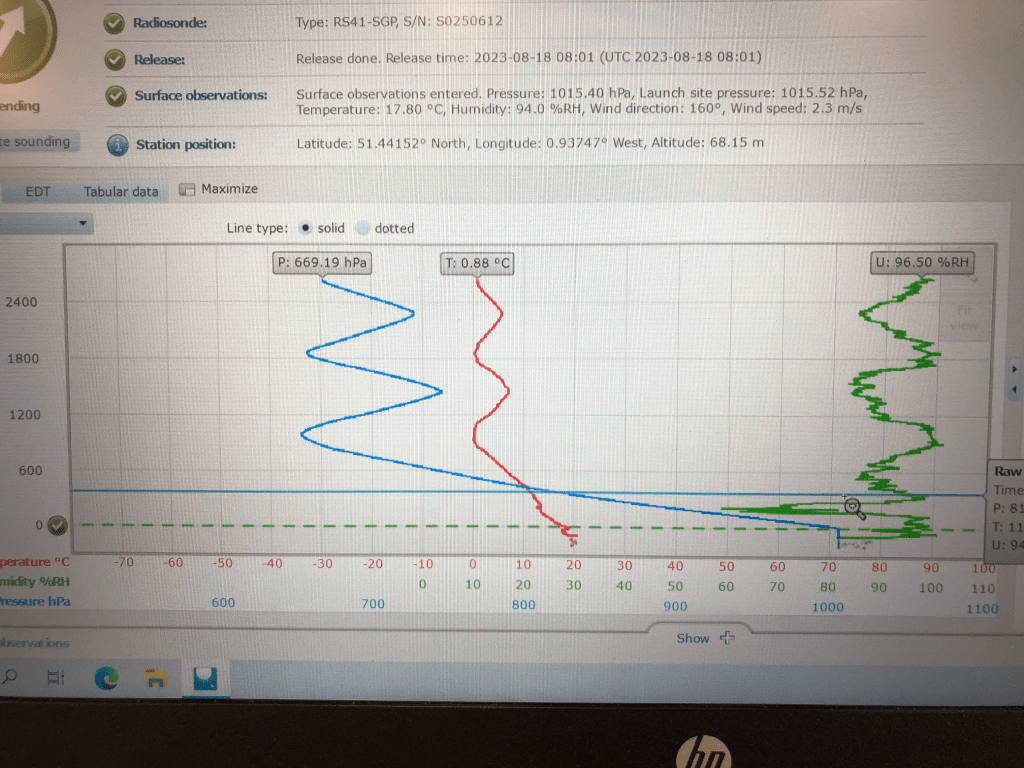
“The wiggler”! Oscillating radiosondes observed during elevated convection events.

Cue the excited discussions trying to explain what we were seeing. Sensor malfunction? Strong downdraughts? Not quite. 

Notice that the peak of each oscillation occurs almost exactly at 0°C. Surely that can’t be coincidental! Turns out these “wiggly” radiosondes have been observed before, albeit infrequently, and is attributed to snow building up on the surface of the balloon, weighing it down. As the balloon sinks and returns to above-freezing temperatures, the accumulated snow gradually melts and departs the balloon, allowing it to rise back up to the freezing level and accumulate more snow, and so on. 

That sounds reasonable enough. So why, then, do we see this oscillating behaviour so infrequently? One of the reasons discovered was purely technical. 

If you would like to read more about these events, a paper is currently being prepared by Stephen Burt, Caleb Miller and Brian Lo. Check back on the blog for further updates!

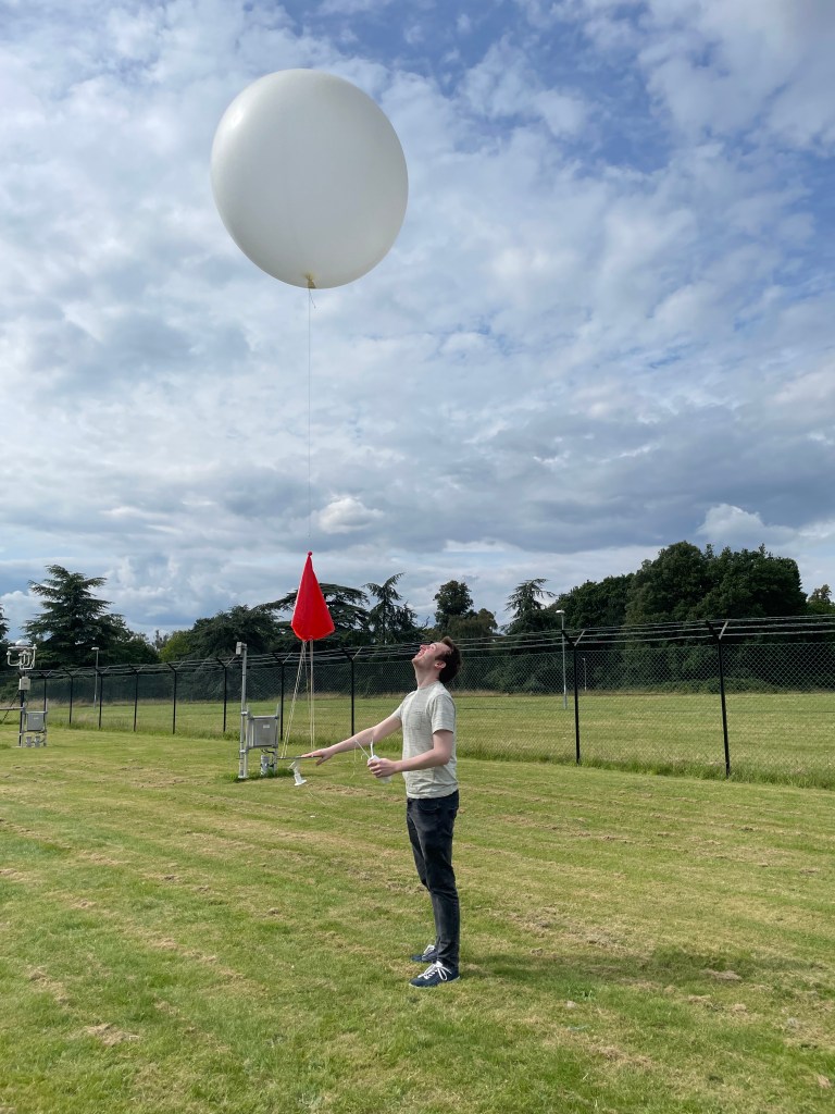
Humphrey Lean, Eme Dean-Lewis (left) and myself (right) ready to launch a sonde.

Met Office Summer Testbed

While not strictly a part of WesCon, this summer’s Met Office testbed was closely connected to the themes of the field campaign, and features plenty of collaboration. 

Testbeds are an opportunity for operational meteorologists, researchers, academics, and even students to evaluate forecast outputs and provide feedback on particular model issues. This year’s testbed was focussed on two main themes: convection and ensembles. These are both high priority areas for development in the Met Office, and the testbed provides a chance to get a broader, more subjective evaluation of these issues.

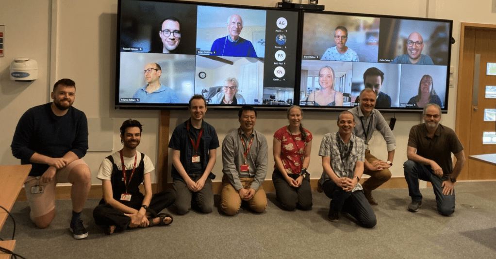
Group photo of the week 2 testbed participants.

Each day was structured into six sets of activities. Firstly, we were divided into three groups to perform a “Forecast Denial Experiment”, whereby each group is given access to a limited set of data and asked to issue a forecast for later in the day. One group only had access to the deterministic UKV model outputs, another group only had access to the MOGREPS-UK high-resolution ensemble output, and the third group has access to both datasets. The idea was to test whether ensemble outputs provide added value and accuracy to forecasts of impactful weather compared to just deterministic outputs. Each group was led by one or two operational meteorologists who navigated the data and, generally, provided most of the guidance. Personally, I found it immensely useful to shadow the op-mets as they made their forecasts, and came away with a much better understanding of the processes which goes into issuing a forecast.

After lunch, we would begin the ensemble evaluation activity which focussed on subjectively evaluating the spread of solutions in the high-resolution MOGREPS-UK ensemble. Improving ensemble spread is one of the major priorities for model development; currently, the members of high-resolution ensembles tend to diverge from the control member too slowly, leading to overconfident forecasts. It was particularly interesting to compare the spread results from MOGREPS-UK with the global MOGREPS-G ensemble and to try to understand the situations when the UK ensemble seemed to resemble a downscaled version of the global model. Next, we would evaluate three surface water flooding products, all combining ensemble data with other surface and impact libraries to produce flooding risk maps. Despite being driven by the same underlying model outputs, it was surprising how much each model differed in the case studies we looked at. 

Finally, we would end the day by evaluating the WMV (Wessex Model Variable) 300 m test ensemble, run over the greater Bristol area over this summer for research purposes. Also driven by MOGREPS-UK, this ensemble would often pick out convective structure which MOGREPS-UK was too coarse to resolve, but also tended to overdo the intensities. It was also very interesting to see the objective metrics suggested that WMV had much worse spread than MOGREPS-UK over the same area, a surprising result which didn’t align with my own interpretation of model performance.

Overall, the testbed was a great opportunity to learn more about how forecasts are issued and to get a deeper intuition for how to interpret model outputs. As researchers, it’s easy to look at model outputs as just abstract data, which is there to be verified and scrutinised, forgetting the impacts that it can have on the people experiencing it. While it was an admittedly exhausting couple of weeks, I would highly recommend more students take part in future testbeds!

Island convection and its many shapes and forms: a closer look at cloud trails

Despite decades of research, convection continues to be one of the major sources of uncertainty in weather and climate models. This is because convection occurs across scales that are smaller than the numerical grids used to integrate these models – in other words, the convection is not resolved in the model. However, its role in the vertical transport of heat, moisture, and momentum could still be important for phenomena that are resolved so the impact of convection is estimated from a set of diagnosed parameters (i.e. a parameterisation scheme).

As the community moves toward modelling with smaller numerical grids, convection can be partially resolved. This numerical regime consisting of partially resolved convection is sometimes called the ‘Convection Grey Zone’. New parameterisations for convection are required for the convection grey zone as the underlying assumptions for existing parameterisations are no longer valid.

With smaller grid spacing, other important processes are better represented – for example, the interaction with the surface. In some coarse climate models, many islands are so small that they are neglected altogether. We know that islands regularly force different kinds of convection and so they offer a real-world opportunity to study the kind of locally driven convection that can now be resolved in operational weather models. My thesis aims to take existing research on small islands a step further by considering the problem from the perspective of convection parameterisation.

Bermuda_DEM
Figure 1. Topographic map of Bermuda showing the coastline in blue, elevation above sea level in grey shading, and the highest elevation is marked by a red triangle.

Bermuda (where I’m from) is a small, relatively flat island located in the western North Atlantic Ocean (e.g. Fig. 1). Cloud trails (CT) here have been unwittingly incorporated into a local legend surrounding an 18th century heist during the American Revolution. This plot to steal British gunpowder to help the American revolutionaries involved the American merchant ‘Captain Morgan’, whose ghost is said to haunt Bermuda on hot, humid summer evenings when dark cloud looms over the east end of the island. This legend is where the local name for the cloud trail “Morgan’s Cloud” comes from (BWS Glossary, 2019).

This story highlights what a CT might look like from a ground observer – a dark cloud which hangs over one end of the island. In fact, CT could only be observed from the ground until research aircraft became feasible in the 1940s and 50s. Aircraft measurements revealed the internal structure of the CT including an associated plume of warmer, drier air immediately downwind of the island.

In the coming decades, the combination of publicly available high-quality satellite imagery and computing advances introduced new avenues for research. This allowed case studies of one-off events and short satellite climatologies constructed by hand (e.g. Nordeen et al., 2001).

Observed from space, CTs look like bands of cloud that stream downwind of, and appear anchored to, small islands. They can be found downwind of small islands around the world, mainly in the tropics and subtropics.

fig1
Figure 2. (Johnston et al., 2018) Observations from visible satellite imagery showing (a) an example CT, (b) an example NT, and (c) an example obscured scene. Imagery from GOES-13 0.64 micron visible channel. In each instance a wind barb indicating the wind speed (knots) and direction. Full feathers on the wind barbs represent 10 kts, and half feathers 5 kts.

In my thesis, we design an algorithm to automate the objective classification of satellite imagery into one of three categories (Fig. 2): CT, NT (Non-Trail), and OB (Obscured). We find that the algorithm results are comparable to manually classified satellite imagery and can construct a much longer climatology of CT occurrence quickly and objectively (Johnston et al., 2018). The algorithm is applied to satellite imagery of Bermuda for May through October of 2012-2016.

We find that CT occurrence peaks in the afternoon and in July. This highlights the strong link to the solar cycle. Furthermore, radiosonde measurements taken via weather balloon by the Bermuda Weather Service show that cloud base height (which is controlled by the low-level humidity) is too high for NT days. This reduces cloud formation in general and prevents the CT cloud band forming. Meanwhile, large-scale disturbances result in widespread cloud cover on OB days (Johnston et al., 2018).

These observations and measurements can only tell us so much. A case CT day is then used to design numerical experiments to consider poorly observed features of the phenomenon. For example, the interplay between the warm plume, CT circulation, and the clouds themselves. These experiments are completed with very small grid spacing (i.e. 100 m vs. the ~10 km in weather models, and ~50 km in climate models). This allows us to confidently simulate both convection and a small island without the use of parameterisations.

Within the boundary layer which buffers the impacts from surface on the free atmosphere, a circulation forms downwind of the heated island. We show that this circulation consists of near-surface convergence, which leads to a band of ascent, and a region of divergence near the top of the boundary layer. This circulation acts as a coherent structure tying the boundary layer to convection in the free atmosphere above.

Further experiments which target the relationship between the island heating, low-level humidity, and wind speed have been completed. These experiments reveal a range of circulation responses. For instance, responses associated with no cloud, mostly passive cloud, and strongly precipitating cloud can result.

We are now using the set of CT experiments to develop a set of expectations upon which existing and future convection parameterisation schemes can be tested and evaluated. We plan to use a selection of the CT experiments with grid spacing increased to values consistent with current operational grey zone models. We believe that this will help to highlight deficiencies in existing parameterisation schemes and focus efforts for the improvement of future schemes.

Further Reading:

Bermuda Weather Service (BWS) Glossary, accessed 2019: Morgan’s Cloud/Morgan’s Cloud (Story). https://www.weather.bm/glossary/glossary.asp

Johnston, M. C., C. E. Holloway, and R. S. Plant, 2018: Cloud Trails Past Bermuda: A Five-Year Climatology from 2012-2016. Mon. Wea. Rev., 146, 4039-4055, https://doi.org/10.1175/MWR-D-18-0141.1

Matthews, S., J. M. Hacker, J. Cole, J. Hare, C. N. Long, and R. M. Reynolds, 2007: Modification of the atmospheric boundary layer by a small island: Observations from Nauru. Mon. Wea. Rev., 135, 891-905, https://doi.org/10.1175/MWR3319.1

Nordeen, M. K., P. Minnis, D. R. Doelling, D. Pethick, and L. Nguyen, 2001: Satellite observations of cloud plumes generated by Nauru. Geophys. Res. Lett., 28, 631-634, https://doi.org/10.1029/2000GL012409

Representing the organization of convection in climate models

Email: m.muetzelfeldt@pgr.reading.ac.uk

Current generation climate models are typically run with horizontal resolutions of 25–50 km. This means that the models cannot explicitly represent atmospheric phenomena that are smaller than these resolutions. An analogy for this is with the resolution of a camera: in a low-resolution, blocky image you cannot make out all the finer details. In the case of climate models, the unresolved phenomena might still be important for what happens at the larger, resolved scales. This is true for convective clouds – clouds such as cumulus and cumulonimbus that are formed from differences in density, caused by latent heat release, between the clouds and the environmental air. Convective clouds are typically around hundreds to thousands of metres in their horizontal size, and so are much smaller than the size of individual grid-columns of a climate model.

Convective clouds are produced by instability in the atmosphere. Air that rises ends up being warmer, and so less dense, than the air that surrounds it, due to the release of latent heat as water is formed by the condensation of water vapour. The heating they produce acts to reduce this instability, leading to a more stable atmosphere. To ensure that this stabilizing effect is included in climate model simulations, convective clouds are represented through what is called a convection parametrization scheme – the stabilization is boiled down to a small number of parameters that model how the clouds act to reduce the instability in a given grid-column. The parametrization scheme then models the action of the clouds in a grid-column by heating the atmosphere higher up, which reduces the instability.

Convection parametrization schemes work by making a series of assumptions about the convective clouds in each grid-column. These include the assumption that there will be many individual convective clouds in grid-columns where convection is active (Fig. 1), and that these clouds will only interact through stabilizing a shared environment. However, in nature, many forms of convective organization are observed, which are not currently represented by convection parametrization schemes.

Figure 1: From Arakawa and Schubert, 1974. Cloud field with many clouds in it – each interacting with each other only by modifying a shared environment.

In my PhD, I am interested in how vertical wind shear can cause the organization of convective cloud fields. Wind shear occurs when the wind is stronger at one height than another. When there is wind shear in the lower part of the atmosphere – the boundary layer – it can organize individual clouds into much larger cloud groups. An example of this is squall lines, which are often seen over the tropics and in mid-latitudes over the USA and China. Squall lines are a type of Mesoscale Convective System (MCS), which account for a large part of the total precipitation over the tropics – between 50 – 80 %. Including their effects in a climate model can therefore have an impact of the distribution of precipitation over the tropics, which is one area where there are substantial discrepancies between climate models and observations.

The goal of my PhD is to work out how to represent shear-induced organization of cloud fields in a climate model’s convection parametrization scheme. The approach I am taking is as follows. First, I need to know where in the climate model the organization of convection is likely to be active. To do this, I have developed a method for examining all of the wind profiles that are produced by the climate model over the tropics, and grouping these into a set of 10 wind profiles that are probably associated with the organization of convection. The link between organization and each grid-column is made by checking that the atmospheric conditions have enough instability to produce convective clouds, and that there is enough low-level shear to make organization likely to happen. With these wind profiles in hand, where they occur can be worked out (Fig. 2 shows the distribution for one of these profiles). The distributions can be compared with distributions of MCSs from satellite observations, and the similarities between the distributions builds confidence that the method is finding wind profiles that are associated with the organization of convection.

Figure 2: Geographical distribution of one of the 10 wind profiles that represents where organization is likely to occur over the tropics. The profile shows a high degree of activity in the north-west tropical Pacific, an area where organization of convection also occurs. This region can be matched to an area of high MCS activity from a satellite derived climatology produced by Mohr and Zipser, 1996.

Second, with these profiles, I can run a set of high-resolution idealized models. The purpose of these is to check that the wind profiles do indeed cause the organization of convection, then to work out a set of relationships that can be used to parametrize the organization that occurs. Given the link between low-level shear and organization, it seems like a good place to start is to check that this link appears in my experiments. Fig. 3 shows the correlation between the low-level shear, and a measure of organization. A clear relationship is seen to hold between these two variables, providing a simple means of parametrizing the degree of organization from the low-level shear in a grid-column.

Figure 3: Correlation of low-level shear (LLS) against a measure of organization (cluster_index). A high degree of correlation is seen, and r-squared values close to 1 indicate that a lot of the variance of cluster_index is explained by the LLS. A p-value of less than 0.001 indicates this is unlikely to have occurred by chance.

Finally, I will need to modify a convection parametrization scheme in light of the relationships that have been uncovered and quantified. To do this, the way that the parametrization scheme models the convective cloud field must be changed to reflect the degree of organization of the clouds. One way this could be done would be by changing the rate at which environmental air mixes into the clouds (the entrainment rate), based on the amount of organization predicted by the new parametrization. From the high-resolution experiments, the strength of the clouds was also seen to be related to the degree of organization, and this implies that a lower value for the entrainment rate should be used when the clouds are organized.

The proof of the pudding is, as they say, in the eating. To check that this change to a parametrization scheme produces sensible changes to the climate model, it will be necessary to make the changes and to run the model. Then the differences in, for example, the distribution of precipitation between the control and the changed climate model can be tested. The hope is then that the precipitation distributions in the changed model will agree more closely with observations of precipitation, and that this will lead to increased confidence that the model is representing more of the aspects of convection that are important for its behaviour.

  • Arakawa, A., & Schubert, W. H. (1974). Interaction of a cumulus cloud ensemble with the large-scale environment, Part I. Journal of the Atmospheric Sciences, 31(3), 674-701.
  • Mohr, K. I., & Zipser, E. J. (1996). Mesoscale convective systems defined by their 85-GHz ice scattering signature: Size and intensity comparison over tropical oceans and continents. Monthly Weather Review, 124(11), 2417-2437.