Island convection and its many shapes and forms: a closer look at cloud trails

Despite decades of research, convection continues to be one of the major sources of uncertainty in weather and climate models. This is because convection occurs across scales that are smaller than the numerical grids used to integrate these models – in other words, the convection is not resolved in the model. However, its role in the vertical transport of heat, moisture, and momentum could still be important for phenomena that are resolved so the impact of convection is estimated from a set of diagnosed parameters (i.e. a parameterisation scheme).

As the community moves toward modelling with smaller numerical grids, convection can be partially resolved. This numerical regime consisting of partially resolved convection is sometimes called the ‘Convection Grey Zone’. New parameterisations for convection are required for the convection grey zone as the underlying assumptions for existing parameterisations are no longer valid.

With smaller grid spacing, other important processes are better represented – for example, the interaction with the surface. In some coarse climate models, many islands are so small that they are neglected altogether. We know that islands regularly force different kinds of convection and so they offer a real-world opportunity to study the kind of locally driven convection that can now be resolved in operational weather models. My thesis aims to take existing research on small islands a step further by considering the problem from the perspective of convection parameterisation.

Bermuda_DEM
Figure 1. Topographic map of Bermuda showing the coastline in blue, elevation above sea level in grey shading, and the highest elevation is marked by a red triangle.

Bermuda (where I’m from) is a small, relatively flat island located in the western North Atlantic Ocean (e.g. Fig. 1). Cloud trails (CT) here have been unwittingly incorporated into a local legend surrounding an 18th century heist during the American Revolution. This plot to steal British gunpowder to help the American revolutionaries involved the American merchant ‘Captain Morgan’, whose ghost is said to haunt Bermuda on hot, humid summer evenings when dark cloud looms over the east end of the island. This legend is where the local name for the cloud trail “Morgan’s Cloud” comes from (BWS Glossary, 2019).

This story highlights what a CT might look like from a ground observer – a dark cloud which hangs over one end of the island. In fact, CT could only be observed from the ground until research aircraft became feasible in the 1940s and 50s. Aircraft measurements revealed the internal structure of the CT including an associated plume of warmer, drier air immediately downwind of the island.

In the coming decades, the combination of publicly available high-quality satellite imagery and computing advances introduced new avenues for research. This allowed case studies of one-off events and short satellite climatologies constructed by hand (e.g. Nordeen et al., 2001).

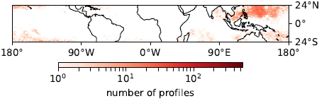
Observed from space, CTs look like bands of cloud that stream downwind of, and appear anchored to, small islands. They can be found downwind of small islands around the world, mainly in the tropics and subtropics.

fig1
Figure 2. (Johnston et al., 2018) Observations from visible satellite imagery showing (a) an example CT, (b) an example NT, and (c) an example obscured scene. Imagery from GOES-13 0.64 micron visible channel. In each instance a wind barb indicating the wind speed (knots) and direction. Full feathers on the wind barbs represent 10 kts, and half feathers 5 kts.

In my thesis, we design an algorithm to automate the objective classification of satellite imagery into one of three categories (Fig. 2): CT, NT (Non-Trail), and OB (Obscured). We find that the algorithm results are comparable to manually classified satellite imagery and can construct a much longer climatology of CT occurrence quickly and objectively (Johnston et al., 2018). The algorithm is applied to satellite imagery of Bermuda for May through October of 2012-2016.

We find that CT occurrence peaks in the afternoon and in July. This highlights the strong link to the solar cycle. Furthermore, radiosonde measurements taken via weather balloon by the Bermuda Weather Service show that cloud base height (which is controlled by the low-level humidity) is too high for NT days. This reduces cloud formation in general and prevents the CT cloud band forming. Meanwhile, large-scale disturbances result in widespread cloud cover on OB days (Johnston et al., 2018).

These observations and measurements can only tell us so much. A case CT day is then used to design numerical experiments to consider poorly observed features of the phenomenon. For example, the interplay between the warm plume, CT circulation, and the clouds themselves. These experiments are completed with very small grid spacing (i.e. 100 m vs. the ~10 km in weather models, and ~50 km in climate models). This allows us to confidently simulate both convection and a small island without the use of parameterisations.

Within the boundary layer which buffers the impacts from surface on the free atmosphere, a circulation forms downwind of the heated island. We show that this circulation consists of near-surface convergence, which leads to a band of ascent, and a region of divergence near the top of the boundary layer. This circulation acts as a coherent structure tying the boundary layer to convection in the free atmosphere above.

Further experiments which target the relationship between the island heating, low-level humidity, and wind speed have been completed. These experiments reveal a range of circulation responses. For instance, responses associated with no cloud, mostly passive cloud, and strongly precipitating cloud can result.

We are now using the set of CT experiments to develop a set of expectations upon which existing and future convection parameterisation schemes can be tested and evaluated. We plan to use a selection of the CT experiments with grid spacing increased to values consistent with current operational grey zone models. We believe that this will help to highlight deficiencies in existing parameterisation schemes and focus efforts for the improvement of future schemes.

Further Reading:

Bermuda Weather Service (BWS) Glossary, accessed 2019: Morgan’s Cloud/Morgan’s Cloud (Story). https://www.weather.bm/glossary/glossary.asp

Johnston, M. C., C. E. Holloway, and R. S. Plant, 2018: Cloud Trails Past Bermuda: A Five-Year Climatology from 2012-2016. Mon. Wea. Rev., 146, 4039-4055, https://doi.org/10.1175/MWR-D-18-0141.1

Matthews, S., J. M. Hacker, J. Cole, J. Hare, C. N. Long, and R. M. Reynolds, 2007: Modification of the atmospheric boundary layer by a small island: Observations from Nauru. Mon. Wea. Rev., 135, 891-905, https://doi.org/10.1175/MWR3319.1

Nordeen, M. K., P. Minnis, D. R. Doelling, D. Pethick, and L. Nguyen, 2001: Satellite observations of cloud plumes generated by Nauru. Geophys. Res. Lett., 28, 631-634, https://doi.org/10.1029/2000GL012409

Investigating the use of early satellite data to test historical reconstructions of sea surface temperature

Email: t.hall@pgr.reading.ac.uk

Observations of sea surface temperature (SST) form one of the key components of the climate record. There are a number of different in-situ based reconstructions of SST extending back over 150 years, but they are not truly independent of each other because the observations they are based on are largely the same (Berry et al., 2018). Datasets of SST retrieved from satellite radiometers exist for the 1980s onwards, providing an independent record of SST. Before this, SST reconstructions are based on sparse, ship-based measurements.

There were meteorological measurements being made from satellites in the 1960s and 70s, however, some of which can potentially be used to retrieve SST. My PhD focuses on investigating if we can retrieve SST from one of these early satellite instruments, to test the reliability of the SST reconstructions before the 1980s. This instrument is the Infrared Interferometer Spectrometer (IRIS), which made measurements of atmospheric emission spectra on-board the Nimbus 4 satellite from April 1970 to January 1971. IRIS had over 800 thermal infrared (IR) channels, covering the 400-1600 cm-1 spectral region. Figure 1 shows an example of two typical IRIS radiance spectra, with the main spectral absorption features labelled as well as the atmospheric window regions, which are the main spectral regions used for SST retrieval.

blog_fig1
Figure 1: Example of two typical IRIS radiance spectra; the main spectral absorption features are labelled as well as the atmospheric window regions.

Before using the IRIS data to retrieve SST, it was necessary to apply a series of quality assurance tests to filter out bad data. A few months into my PhD, work by Bantges et al. (2016) revealed evidence for a wavelength dependent cold bias of up to 2K in the data. A large part of my PhD was spent trying to quantify this bias. This was done by comparing clear-sky IRIS spectra with spectra simulated with a radiative transfer model. Unfortunately, this meant that the SSTs eventually retrieved from IRIS are not totally independent of the SST reconstructions as the simulations are based on reanalysis data forced by the HadISST2 reconstruction. Figure 2 compares our estimate of the IRIS spectral bias with globally averaged spectral differences between IRIS, the Interferometric Monitor for Greenhouse Gases (IMG) and the Infrared Atmospheric Sounding Instrument (IASI) from Bantges et al. (2016). This shows close agreement between our bias estimate and the IRIS-IMG and IRIS-IASI differences outside of the ozone spectral region, which is not relevant for SST retrieval.

It cannot just be assumed that the bias is the same for each IRIS measurement. Comparison of IRIS (bias-corrected using our initial bias estimate) with window channel data from the Temperature-Humidity Infrared Radiometer (THIR), also on-board Nimbus 4, reveals that the relative IRIS-THIR bias varies with window brightness temperature and orbit angle. The THIR, however, may have biases of its own, so these biases cannot be attributed to IRIS.

blog_fig2
Figure 2: Area-weighted global mean brightness temperature difference averaged over AMJ between IRIS (1970), IMG (1997) and IASI (2012) (black and blue lines) from Bantges et al. (2016), compared with our IRIS bias estimate, also area-weighted and averaged over AMJ (red line). The ozone absorption band is not used for SST retrieval, so is shaded grey.

The technique of optimal estimation was applied to retrieve SST from IRIS. This uses the observation-simulation differences together with information about the sensitivity of the simulations to the state of the atmosphere and ocean to estimate the SST. IR satellite retrievals of SST are usually performed in clear-sky conditions only. However, the low spatial resolution of IRIS means that very few cases are fully clear-sky. For this reason, we had to adapt the retrieval method to be tolerant of some cloud. This involves retrieving SST simultaneously with cloud fraction (CF). The retrieval method was then tested on partly cloudy (≤0.2 CF) IASI spectra made ‘IRIS-like’ by spatial averaging, spectral smoothing and simulating IRIS-like errors. The retrieved IRIS-like SSTs were validated against quality-controlled drifting buoy SSTs. This revealed latitudinal biases in the retrieved SSTs for the partly cloudy cases, not present in the SSTs for clear-sky cases.

SSTs were then retrieved for all IRIS cases with an expected CF ≤ 0.2. Figure 3 shows the difference between the gridded, monthly average IRIS SSTs and two of the SST reconstructions (HadSST3 and HadISST2) for July 1970. There are large, spatially correlated differences between the IRIS SSTs and reconstructions. We expect a latitudinal bias in the IRIS SSTs and some level of remaining bias in the IRIS spectra is likely, contributing to further SST bias. It is therefore likely that the differences in Figure 3 are mainly due to bias in the IRIS SSTs rather than the reconstructions.

iris_recon_07_70
Figure 3: Gridded IRIS-HadSST3 (left) and IRIS-HadISST2 (right) SST for July 1970. HadISST2 is a globally complete, interpolated dataset whereas HadSST3 is not globally complete.

Despite being unable to retrieve bias-free SST estimates from IRIS, my work has contributed towards better understanding the characteristics of IRIS. This ties in with a current project aiming to recover and assess the quality of data from a number of different historic satellite sensors, including IRIS, for assimilation in the next generation of climate reanalyses.

References

Bantges, R., H. Brindley, X. H. Chen, X. L. Huang, J. Harries, J. Murray (2016), On the detection of robust multi-decadal changes in the Earth’s Outgoing Longwave Radiation spectrum. J. Climate, 29, 4939-4947. https://doi.org/10.1175/JCLI-D-15-0713.1

Berry, D. I., G. K. Corlett, O. Embury, C. J. Merchant (2018), Stability assessment of the (A)ATSR Sea Surface Temperature climate dataset from the European Space Agency Climate Change Initiative. Remote Sens., 10, 126. https://doi.org/10.3390/rs10010126

EGU 2019

From 7th-12th April, I had the exciting opportunity to attend the European Geosciences Union (EGU) General Assembly in Vienna. This was a much larger conference than any I had attended previously, with 16,273 scientists in attendance and 683 scientific sessions, which made for a whirlwind experience. I was staying with other PhD students from the department, so many evenings were spent comparing schedules and pointing out interesting courses to make sure none of us missed anything useful!

As part of the Tropical Meteorology and Tropical Cyclones session, I gave an oral presentation about my PhD work, which investigates the use of Available Potential Energy theory to study the processes involved in tropical cyclone intensification. The session included many excellent talks on different aspects of tropical meteorology, and it was great to speak with scientists whose interests are similar to mine about possible avenues for combining our work.

PhD students from the department present their research at EGU

One of the major advantages of attending such a large conference was the opportunity to learn more about areas of geoscience research that I wouldn’t normally encounter. I made a specific effort to attend a few sessions on topics that I am not familiar with, including wildfires (#FIREMIP), landslides and exoplanets. It was fascinating to see the work that goes on in different fields and I hope that being exposed to different methods and perspectives will help me to become a more creative researcher.

EGU is such a huge event that the scientific sessions are only part of the story. There were Great Debates on topics ranging from science in policy to the prioritisation of mental wellbeing for Early Career Scientists, two artists-in-residence creating pieces inspired by the science of the conference, and an extremely entertaining Poetry Slam event, which two of the Reading Meteorology PhD students were brave enough to participate in (or possibly just desperate enough for a ticket to the conveners’ party).

poetry

So now it’s the end of EGU
I caught the train – and I flew
We both did a talk
Learnt the German for fork
“Eine Gabel bitte” – thank you

– Sally Woodhouse & Kaja Milczewska

EGU was a great experience and after the conference I was able to take some time to explore Vienna, see some historic landmarks, and unwind from an enjoyably exhausting week of science. Although to begin my break from geoscience I did go straight to the Globe Museum, so perhaps I need to work on my relaxation techniques.


#traintoEGU – Sally Woodhouse

Aviation currently contributes over 2% of the annual global CO2 emissions which, if classed as a country, would make it one of the top ten emitters. A return flight to Vienna from London adds about 0.2 metric tonnes of CO2 to your carbon footprint (the UK annual mean per person is 6.5 metric tonnes).

An important part of science is sharing our research and one of the best ways to do that is at conferences, so we can’t just stop going! But there is another way … the train (0.04 metric tonnes CO2)! And if I’m spending all that time why not have a little adventure.

With the help of the man in seat 61 (check it out if you’re getting the train anywhere it’s so helpful!) we decided to go via Zurich. We had a night’s stop in Zurich, a morning there exploring and then an afternoon train through the stunning Arlberg Pass and beautiful views of Alpine Austria. Honestly the views made the 5am start the day before and sprint for the Eurostar all worth it. It was breath-taking for the whole 8 hour journey.


traintoEGU_Paris_Zurich

For the return trip we took the speedy route through Germany and Belgium – this is actually doable in a day but I decided to have an overnight in Brussels. I spent a lovely day wandering around the main sites and even managed a visit to the European Parliament!

It might take a bit longer but it was a wonderful adventure and I’d definitely recommend it to everyone traveling to EGU in future – maybe I’ll see you on the train.

traintoEGU_Brussels

Representing the organization of convection in climate models

Email: m.muetzelfeldt@pgr.reading.ac.uk

Current generation climate models are typically run with horizontal resolutions of 25–50 km. This means that the models cannot explicitly represent atmospheric phenomena that are smaller than these resolutions. An analogy for this is with the resolution of a camera: in a low-resolution, blocky image you cannot make out all the finer details. In the case of climate models, the unresolved phenomena might still be important for what happens at the larger, resolved scales. This is true for convective clouds – clouds such as cumulus and cumulonimbus that are formed from differences in density, caused by latent heat release, between the clouds and the environmental air. Convective clouds are typically around hundreds to thousands of metres in their horizontal size, and so are much smaller than the size of individual grid-columns of a climate model.

Convective clouds are produced by instability in the atmosphere. Air that rises ends up being warmer, and so less dense, than the air that surrounds it, due to the release of latent heat as water is formed by the condensation of water vapour. The heating they produce acts to reduce this instability, leading to a more stable atmosphere. To ensure that this stabilizing effect is included in climate model simulations, convective clouds are represented through what is called a convection parametrization scheme – the stabilization is boiled down to a small number of parameters that model how the clouds act to reduce the instability in a given grid-column. The parametrization scheme then models the action of the clouds in a grid-column by heating the atmosphere higher up, which reduces the instability.

Convection parametrization schemes work by making a series of assumptions about the convective clouds in each grid-column. These include the assumption that there will be many individual convective clouds in grid-columns where convection is active (Fig. 1), and that these clouds will only interact through stabilizing a shared environment. However, in nature, many forms of convective organization are observed, which are not currently represented by convection parametrization schemes.

Figure 1: From Arakawa and Schubert, 1974. Cloud field with many clouds in it – each interacting with each other only by modifying a shared environment.

In my PhD, I am interested in how vertical wind shear can cause the organization of convective cloud fields. Wind shear occurs when the wind is stronger at one height than another. When there is wind shear in the lower part of the atmosphere – the boundary layer – it can organize individual clouds into much larger cloud groups. An example of this is squall lines, which are often seen over the tropics and in mid-latitudes over the USA and China. Squall lines are a type of Mesoscale Convective System (MCS), which account for a large part of the total precipitation over the tropics – between 50 – 80 %. Including their effects in a climate model can therefore have an impact of the distribution of precipitation over the tropics, which is one area where there are substantial discrepancies between climate models and observations.

The goal of my PhD is to work out how to represent shear-induced organization of cloud fields in a climate model’s convection parametrization scheme. The approach I am taking is as follows. First, I need to know where in the climate model the organization of convection is likely to be active. To do this, I have developed a method for examining all of the wind profiles that are produced by the climate model over the tropics, and grouping these into a set of 10 wind profiles that are probably associated with the organization of convection. The link between organization and each grid-column is made by checking that the atmospheric conditions have enough instability to produce convective clouds, and that there is enough low-level shear to make organization likely to happen. With these wind profiles in hand, where they occur can be worked out (Fig. 2 shows the distribution for one of these profiles). The distributions can be compared with distributions of MCSs from satellite observations, and the similarities between the distributions builds confidence that the method is finding wind profiles that are associated with the organization of convection.

Figure 2: Geographical distribution of one of the 10 wind profiles that represents where organization is likely to occur over the tropics. The profile shows a high degree of activity in the north-west tropical Pacific, an area where organization of convection also occurs. This region can be matched to an area of high MCS activity from a satellite derived climatology produced by Mohr and Zipser, 1996.

Second, with these profiles, I can run a set of high-resolution idealized models. The purpose of these is to check that the wind profiles do indeed cause the organization of convection, then to work out a set of relationships that can be used to parametrize the organization that occurs. Given the link between low-level shear and organization, it seems like a good place to start is to check that this link appears in my experiments. Fig. 3 shows the correlation between the low-level shear, and a measure of organization. A clear relationship is seen to hold between these two variables, providing a simple means of parametrizing the degree of organization from the low-level shear in a grid-column.

Figure 3: Correlation of low-level shear (LLS) against a measure of organization (cluster_index). A high degree of correlation is seen, and r-squared values close to 1 indicate that a lot of the variance of cluster_index is explained by the LLS. A p-value of less than 0.001 indicates this is unlikely to have occurred by chance.

Finally, I will need to modify a convection parametrization scheme in light of the relationships that have been uncovered and quantified. To do this, the way that the parametrization scheme models the convective cloud field must be changed to reflect the degree of organization of the clouds. One way this could be done would be by changing the rate at which environmental air mixes into the clouds (the entrainment rate), based on the amount of organization predicted by the new parametrization. From the high-resolution experiments, the strength of the clouds was also seen to be related to the degree of organization, and this implies that a lower value for the entrainment rate should be used when the clouds are organized.

The proof of the pudding is, as they say, in the eating. To check that this change to a parametrization scheme produces sensible changes to the climate model, it will be necessary to make the changes and to run the model. Then the differences in, for example, the distribution of precipitation between the control and the changed climate model can be tested. The hope is then that the precipitation distributions in the changed model will agree more closely with observations of precipitation, and that this will lead to increased confidence that the model is representing more of the aspects of convection that are important for its behaviour.

  • Arakawa, A., & Schubert, W. H. (1974). Interaction of a cumulus cloud ensemble with the large-scale environment, Part I. Journal of the Atmospheric Sciences, 31(3), 674-701.
  • Mohr, K. I., & Zipser, E. J. (1996). Mesoscale convective systems defined by their 85-GHz ice scattering signature: Size and intensity comparison over tropical oceans and continents. Monthly Weather Review, 124(11), 2417-2437.

Workshop on Predictability, dynamics and applications research using the TIGGE and S2S ensembles

Email: s.h.lee@pgr.reading.ac.uk

From April 2nd-5th I attended the workshop on Predictability, dynamics and applications research using the TIGGE and S2S ensembles at ECMWF in Reading. TIGGE (The International Grand Global Ensemble, formerly THORPEX International Grand Global Ensemble) and S2S (Sub-seasonal-to-Seasonal) are datasets hosted at primarily at ECMWF as part of initiatives by the World Weather Research Programme (WWRP) and the World Climate Research Programme (WCRP). TIGGE has been running since 2006 and stores operational medium-range forecasts (up to 16 days) from 10 global weather centres, whilst S2S has been operational since 2015 and houses extended-range (up to 60 days) forecasts from 11 different global weather centres (e.g. ECMWF, NCEP, UKMO, Meteo-France, CMA…etc.). The benefit of these centralised datasets is their common format, which enables straightforward data requests and multi-model analysis with minimal data manipulation allowing scientists to focus on doing science!

Attendees of the workshop came from around the world (not just Europe) although there was a particularly sizeable cohort from Reading Meteorology and NCAS.

Figure 1: Workshop group photo featuring the infamous ECMWF ducks!

In my PhD so far, I have been making extensive use of the S2S database – looking at both operational and re-forecast datasets to assess stratospheric predictability and biases – and it was rewarding to attend the workshop and see what a diverse range of applications the datasets have across the world. From the oceans to the stratosphere, tropics to poles, predictability mathematics to farmers and energy markets, it was immediately very clear that TIGGE and S2S are wonderfully useful tools for both the research and applications communities. A particular aim of the workshop was to discuss “user-oriented variables” – derived variables from model output which represent the meteorological conditions to which a user is sensitive (such as wind speed at a specific height for wind power applications).

The workshop mainly consisted of 15-minute conference-style talks in the main lecture theatre and poster sessions, but the final two days also featured parallel working group sessions of about 15 members each. The topics discussed in the working groups can be found here. I was part of working group 4, and we discussed dynamical processes and ensemble diagnostics. We reflected on some of the points raised by speakers over the preceding days – particular attention was given to diagnostics needed to understand dynamical effects of model biases (such as their influence on Rossby wave propagation and weather-regime transition) alongside what other variables researchers needed to make full use of the potentials S2S and TIGGE offer (I don’t think I could say “more levels in the stratosphere!” loudly enough – TIGGE does not go above 50 hPa, which is not useful when studying stratospheric warming events defined at 10 hPa).

Data analysis tools are also becoming increasingly important in atmospheric science. Several useful and perhaps less well-known tools were presented at the workshop – Mio Matsueda’s TIGGE and S2S museum websites provide a wide variety of pre-prepared plots of variables like the NAO and MJO which are excellent for exploratory data analysis without needing many gigabytes of data downloads. Figure 2 shows an example of NAO forecasts from S2S data – the systematic negative NAO bias at longer lead-times was frequently discussed during the workshop, whilst the inability to capture the transition to a positive NAO regime beginning around February 10th is worth further analysis. In addition to these, IRI’s Data Library has powerful abilities to manipulate, analyse, plot, and download data from various sources including S2S with server-side computation.


Figure 2: Courtesy of the S2S Museum, this figure shows S2S model forecasts of the NAO launched on January 31st 2019. The verifying scenario is shown in black, with ensemble means in grey. All models exhibited a negative ensemble-mean bias and did not capture the development of a positive NAO after February 10th.

It’s inspiring and motivating to be part of the sub-seasonal forecast research community and I’m excited to present some of my work in the near future!

TIGGE and S2S can be accessed via ECMWF’s Public Datasets web interface.

On relocating to the Met Office for five weeks of my PhD

Some PhD projects are co-organised by an industrial CASE partner which provides supervisory support and additional funding. As part of my CASE partnership with the UK Met Office, in January I had the opportunity to spend 5 weeks at the Exeter HQ, which proved to be a fruitful experience. As three out of my four supervisors are based there, it was certainly a convenient set-up to seek their expertise on certain aspects of my PhD project!

One part of my project aims to understand how certain neighbourhood-based verification methods can affect the level of surface air quality forecast accuracy. Routine verification of a forecast model against observations is necessary to provide the most accurate forecast possible. Ensuring that this happens is crucial, as a good forecast may help keep the public aware of potential adverse health risks resulting from elevated pollutant concentrations.

The project deals with two sides of one coin: evaluating forecasts of regional surface pollutant concentrations; and evaluating those of meteorological fields such as wind speed, precipitation, relative humidity or temperature. All of the above have unique characteristics: they vary in resolution, spatial scale, homogeneity, randomness… The behaviour of the weather and pollutant variables is also tricky to compare against one another because the locations of their numerous measurement sites nearly never coincide, whereas the forecast encompasses the entirety of the domain space. This is kind of the crux of this part of my PhD: how can we use these irregularly located measurements to our advantage in verifying the skill of the forecast in the most useful way? And – zooming out still – can we determine the extent to which the surface air pollution forecast is dependent on some of those aforementioned weather variables? And can this knowledge (once acquired!) be used to further improve the pollution forecast?

IMG_4407
Side view of the UK Met Office on a cold day in February.

While at the Met Office, I began my research specifically into methods which analyse the forecast skill when a model “neighbourhood” of a particular size around a particular point-observation is evaluated. These methods are being developed as part of a toolkit for evaluation of high resolution forecasts, which can be (and usually are) more accurate than a lower resolution equivalent, but traditional metrics (e.g. root mean square error (RMSE) or mean error (ME)) often fail to demonstrate the improvement (Mittermaier, 2014). They can also fall victim to various verification errors such as the double-penalty problem. This is when an ‘event’ might have been missed at a particular time in the forecast at one gridpoint because it was actually forecast in the neighbouring grid-point one time-step out, so the RMSE counts this error both in the spatial and temporal axes. Not fair, if you ask me. So as NWP continues to increase in resolution, there is a need for robust verification methods which relax the spatial (or temporal) restriction on precise forecast-to-observation matching somewhat (Ebert, 2008).

One way to proceed forward is via a ‘neighbourhood’ approach which treats a deterministic forecast almost as an ensemble by considering all the grid-points around an observation as an individual forecast and formulating a probabilistic score. Neighbourhoods are made of varying number of model grid-points, i.e. a 3×3 or a 5×5 or even bigger. A skill score such as the ranked probability score (RPS) or Brier Score is calculated using the cumulative probability distribution across the neighbourhood of the exceedance of a sensible pollutant concentration threshold. So, for example, we can ask what proportion of a 5×5 neighbourhood around an observation has correctly forecasted an observed exceedance (i.e. ‘hit’)? What if an exceedance forecast has been made, but the observed quantity didn’t reach that magnitude (i.e. ‘false alarm’)? And how do these scores change when larger (or smaller) neighbourhoods are considered? And, if these spatial verification methods prove informative, how could they be implemented in operational air quality forecast verification? All these questions will hopefully have some answers in the near future and form a part of my PhD thesis!

Although these kind of methods have been used for meteorological variables, they haven’t yet been widely researched in the context of regional air quality forecasts. The verification framework for this is called HiRA – High Resolution Assessment, which is part of the wider verification network Model Evaluation Tools (which, considering it is being developed as a means of uniformly assessing high-resolution meteorological forecasts, has the most unhelpful acronym: MET). It is quite an exciting opportunity to be involved in the testing and evaluation of this new set of verification tools for a surface pollution forecast at a regional scale, and I am very grateful to be involved in this. Also, having the opportunity to work at the Met Office and “pretend” to be a real research scientist for a while is awesome!

Email: k.m.milczewska@pgr.reading.ac.uk

Extending the predictability of flood hazard at the global scale

Email: rebecca.emerton@reading.ac.uk

When I started my PhD, there were no global scale operational seasonal forecasts of river flow or flood hazard. Global overviews of upcoming flood events are key for organisations working at the global scale, from water resources management to humanitarian aid, and for regions where no other local or national forecasts are available. While GloFAS (the Global Flood Awareness System, run by the European Centre for Medium-Range Weather Forecasts (ECMWF) and the European Commission Joint Research Centre (JRC) as part of the Copernicus Emergency Management Services) was producing operational, openly-available flood forecasts out to 30 days ahead, there was a need for more extended-range forecast information. Often, due to a lack of hydrological forecasts, seasonal rainfall forecasts are used as a proxy for flood hazard – however, the link between precipitation and floodiness is nonlinear, and recent research has shown that seasonal rainfall forecasts are not necessarily the best indicator of potential flood hazard. The aim of my PhD research was to look into ways in which we could provide earlier warning information, several weeks to months ahead, using hydrological analysis in addition to the meteorology.

Presidente Kuczynski recorre zonas afectadas por lluvias e inund
Flooding in Trujillo, Peru, March 2017 (Photo: Presidencia Perú on Twitter)

Broadly speaking, there are two key ways in which to provide early warning information on seasonal timescales: (1) through statistical analysis based on large-scale climate variability and teleconnections, and (2) by producing dynamical seasonal forecasts using coupled ocean-atmosphere GCMs. Over the past 4.5 years, I worked on providing hydrologically-relevant seasonal forecast products using these two approaches, at the global scale. This blog post will give a quick overview of the two new forecast products we produced as part of this research!

Can we use El Niño to predict flood hazard?

ENSO (the El Niño Southern Oscillation), is known to influence river flow and flooding across much of the globe, and often, statistical historical probabilities of extreme precipitation during El Niño and La Niña (the extremes of ENSO climate variability) are used to provide information on likely flood impacts. Due to its global influence on weather and climate, we decided to assess whether it is possible to use ENSO as a predictor of flood hazard at the global scale, by assessing the links between ENSO and river flow globally, and estimating the equivalent historical probabilities for high and low river flow, to those that are already used for meteorological variables.

With a lack of sufficient river flow observations across much of the globe, we needed to use a reanalysis dataset – but global reanalysis datasets for river flow are few and far between, and none extended beyond ~40 years (which includes a sample of ≤10 El Niños and ≤13 La Niñas). We ended up producing a 20th Century global river flow reconstruction, by forcing the Camaflood hydrological model with ECMWF’s ERA-20CM atmospheric reconstruction, to produce a 10-member river flow dataset covering 1901-2010, which we called ERA-20CM-R.

elnino_flood_hazard_gif_beccalize

Using this dataset, we calculated the percentage of past El Niño and La Niña events, during which the monthly mean river flow exceeded a high flow threshold (the 75th percentile of the 110-year climatology) or fell below a low flow threshold (the 25th percentile), for each month of an El Niño / La Niña. This percentage is then taken as the probability that high or low flow will be observed in future El Niño/La Niña events. Maps of these probabilities are shown above, for El Niño, and all maps for both El Niño and La Niña can be found here. When comparing to the same historical probabilities calculated for precipitation, it is evident that additional information can be gained from considering the hydrology. For example, the River Nile in northern Africa is likely to see low river flow, even though the surrounding area is likely to see more precipitation – because it is influenced more by changes in precipitation upstream. In places that are likely to see more precipitation but in the form of snow, there would be no influence on river flow or flood hazard during the time when more precipitation is expected. However, several months later, there may be no additional precipitation expected, but there may be increased flood hazard due to the melting of more snow than normal – so we’re able to see a lagged influence of ENSO on river flow in some regions.

While there are locations where these probabilities are high and can provide a useful forecast of hydrological extremes, across much of the globe, the probabilities are lower and much more uncertain (see here for more info on uncertainty in these forecasts) than might be useful for decision-making purposes.

Providing openly-available seasonal river flow forecasts, globally

For the next ‘chapter’ of my PhD, we looked into the feasibility of providing seasonal forecasts of river flow at the global scale. Providing global-scale flood forecasts in the medium-range has only become possible in recent years, and extended-range flood forecasting was highlighted as a grand challenge and likely future development in hydro-meteorological forecasting.

To do this, I worked with Ervin Zsoter at ECMWF, to drive the GloFAS hydrological model (Lisflood) with reforecasts from ECMWF’s latest seasonal forecasting system, SEAS5, to produce seasonal forecasts of river flow. We also forced Lisflood with the new ERA5 reanalysis, to produce an ERA5-R river flow reanalysis with which to initialise Lisflood, and to provide a climatology. The system set-up is shown in the flowchart below.

glofas_seasonal_flowchart_POSTER_EGU

I also worked with colleagues at ECMWF to design forecast products for a GloFAS seasonal outlook, based on a combination of features from the GloFAS flood forecasts, and the EFAS (the European Flood Awareness System) seasonal outlook, and incorporating feedback from users of EFAS.

After ~1 year of working on getting the system set up and finalising the forecast products, including a four-month research placement at ECMWF, the first GloFAS -Seasonal forecast was released in November 2017, with the release of SEAS5. GloFAS-Seasonal is now running operationally at ECMWF, providing forecasts of high and low weekly-averaged river flow for the global river network, up to 4 months ahead, with 3 new forecast layers available through the GloFAS interface. These provide a forecast overview for 307 major river basins, a map of the forecast for the entire river network at the sub-basin scale, and ensemble hydrographs at thousands of locations across the globe (which change with each forecast depending on forecast probabilities). New forecasts are produced once per month, and released on the 10th of each month. You can find more information on each of the different forecast layers and the system set-up here, and you can access the (openly available) forecasts here. ERA5-R, ERA-20CM-R and the GloFAS-Seasonal reforecasts are also all freely available – just get in touch! GloFAS-Seasonal will continue to be developed by ECMWF and the JRC, and has already been updated to v2.0, including a calibrated version of the hydrological model.

NEW_WEB_figure1_basins
Screenshot of the GloFAS seasonal outlook at www.globalfloods.eu

So, over the course of my PhD, we developed two new seasonal forecasts for hydrological extremes, at the global scale. You may be wondering whether they’re skilful, or in fact, which one provides the most useful forecasts! For information on the skill or ‘potential usefulness’ of GloFAS-Seasonal, head to our paper, and stay tuned for a paper coming soon (hopefully! [update: this paper has just been accepted and can be accessed online here]) on the ‘most useful approach for forecasting hydrological extremes during El Niño’, in which we compare the skill of the two forecasts at predicting observed high and low flow events during El Niño.


With thanks to my PhD supervisors & co-authors:

Hannah Cloke1, Liz Stephens1, Florian Pappenberger2, Steve Woolnough1, Ervin Zsoter2, Peter Salamon3, Louise Arnal1,2, Christel Prudhomme2, Davide Muraro3

1University of Reading, 2ECMWF, 3European Commission Joint Research Centre

The Circumglobal Teleconnection and its Links to Seasonal Forecast Skill for the European Summer

Email: j.beverley@pgr.reading.ac.uk

Recent extreme weather events such as the central European heatwave in 2003, flooding in the UK in 2007, and even the recent dry summer in the UK in 2018, have highlighted the need for more accurate long-range forecasts for the European summer. Recent research has led to improvements in European winter seasonal forecasts, however summer forecast skill remains relatively low. One potential source of predictability for Europe is the Indian summer monsoon, which can affect European weather via a global wave train known as the “Circumglobal Teleconnection” (CGT).

figure1
Figure 1: One-point correlation between 200 hPa geopotential height at the base point (35°-40°N, 60°-70°E) and 200 hPa geopotential height elsewhere in the ERA-Interim (1981–2014) reanalysis dataset, for August. The boxes indicate the regions defined as the “centres of action” of the CGT – these are North Pacific (NPAC), North America (NAM), Northwest Europe (NWEUR), Ding and Wang (D&W) and East Asia (EASIA).

The CGT was first identified by Ding and Wang (2005) as having a major role in modulating observed weather patterns in the Northern Hemisphere summer. Using a 200 hPa geopotential height index centred in west-central Asia (35°-40°N, 60°-70°E), they constructed a one-point correlation map of geopotential height with reference to this index (reproduced in Figure 1). From this, they identified a wavenumber-5 structure where the pressure variations over the Northeast Atlantic, East Asia, North Pacific and North America are all nearly in phase with the variations over west-central Asia (these are known as the “centres of action”). They also showed that the CGT is associated with significant temperature and precipitation anomalies in Europe, so accurate representation this mechanism in seasonal forecast models could provide an important source of subseasonal to seasonal forecast skill.

The model used here is a version of the European Centre for Medium-Range Weather Forecasts (ECMWF)’s coupled seasonal forecast model. Reforecasts are initialised on 1st May and are run for four months, so cover May-August, with start dates from 1981-2014. The skill of the model 200 hPa geopotential height is shown in Figure 2, defined as the correlation between the model ensemble mean and ERA-Interim. The model has good skill in May (to be expected given that the reforecasts are initialised in May) but in June, July and August areas of zero or negative correlation develop across much of the northern hemisphere extratropics. The areas of reduced skill align closely with the location of the centres of action of the CGT shown in Figure 1, suggesting that there is a link between the model skill and the model representation of the CGT.

figure2
Figure 2: Model ensemble mean skill for 200 hPa geopotential height as defined as the correlation between ERA-Interim and model ensemble mean for (a) May (b) June (c) July and (d) August

To determine how well the model represents the CGT, Figure 3 shows the correlation between the D&W region and the other centres of action of the CGT, as defined in Figure 1. Focussing on August (as August has the strongest CGT pattern) it can be seen that the model correlations, indicated by the box and whisker plots, are weaker than in observations (red diamond) for the D&W vs. North Pacific (NPAC), North America (NAM) and Northwest Europe (NWEUR) regions. This indicates that the model has a weak representation of the wavetrain associated with the CGT.

figure3
Figure 3: Distribution of correlation coefficients for the D&W Index correlated against the other centres of action of the CGT. The box plots represent the upper and lower quartiles, and the whiskers extend to the 5th and 95th percentiles. The black horizontal line represents the median value and the red diamond the observed correlation coefficient from ERA-Interim.

There are likely to be several reasons for the weak representation of the CGT in the model. One important factor is the presence of a northerly jet bias in the model across much of the Northern Hemisphere. This can be seen in Figure 4, which shows the model jet biases relative to ERA-Interim in the coloured contours, and the observed zonal wind in the black contours. The dipole structure of the biases which exists across much of the hemisphere, particularly in June, July and August, indicates that the model jet stream is located too far to the north. This means that Rossby waves forced in this region will have different wave propagation characteristics to reality – they may propagate at the incorrect speed, in the wrong direction or may not propagate at all, and this is likely to be an important factor in the weak representation of the CGT in the model.

figure4
Figure 4: Model 200 hPa zonal wind bias (filled contours, m/s), defined as the model ensemble mean minus ERA-Interim zonal wind, and ERA-I 200 hPa zonal wind (black contours) for (a) May (b) June (c) July and (d) August. The location of the centres of action of the CGT are marked with white crosses.

Other potential factors involved are a poor representation of the link between monsoon precipitation and the geopotential height in west-central Asia (which was shown by Ding and Wang (2007) to be important in the maintenance of the CGT) and errors in the forcing of Rossby waves associated with the monsoon. For a more detailed explanation of these, see my paper in Climate Dynamics (Beverley et al. 2018). It seems likely that the pattern of reduced skill in Figure 2, with negative correlations located at the centres of action of the CGT, including over Europe, is related to the poor representation of the CGT in the model. This raises the question of whether an improvement in the model’s representation of the CGT would lead to an improvement in forecast skill for the European summer. To address this question, sensitivity experiments have been carried out, in which the observed circulation is imposed in several centres of action along the CGT pathway to explore the impact on forecast skill for European summer weather.

References

Beverley, J. D., S. J. Woolnough, L. H. Baker, S. J. Johnson and A. Weisheimer, 2018: The northern hemisphere circumglobal teleconnection in a seasonal forecast model and its relationship to European summer forecast skill. Clim. Dyn. https://doi.org/10.1007/s00382-018-4371-4

Ding, Q., and B. Wang, 2005: Circumglobal teleconnection in the northern hemisphere summer. J. Clim. 18, 3483–3505.  https://doi.org/10.1175/JCLI3473.1

Ding, Q., and B. Wang, 2007: Intraseasonal teleconnection between the summer Eurasian wave train and the Indian monsoon. J. Clim. 20, 3751-3767. https://doi.org/10.1175/JCLI4221.1