When the Lakes Remember: Unravelling the Sudd Floods of 2022

By Douglas Mulangwa – d.mulangwa@pgr.reading.ac.uk

Between 2019 and 2024, East Africa experienced one of the most persistent high-water periods in modern history: a flood that simply would not recede. Lakes Victoria, Kyoga, and Albert all rose to exceptional levels, and the Sudd Wetland in South Sudan expanded to an unprecedented 163,000 square kilometres in 2022. More than two million people were affected across Uganda and South Sudan as settlements, roads, and farmland remained inundated for months.

At first, 2022 puzzled stakeholders, observers and scientists alike. Rainfall across much of the region was below average that year, yet flooding in the Sudd intensified. This prompted a closer look at the wider hydrological system. Conventional explanations based on local rainfall failed to account for why the water would not recede. The answer, it turned out, lay far upstream and more than a year earlier, hidden within the White Nile’s connected lakes and wetlands.

Figure 1: Map of the White Nile Basin showing delineated sub-catchments, lakes, major  rivers, and the Sudd Wetland extent. Sub-catchments are labelled numerically (1–15) with names listed in the legend. Observation stations (A–F) mark key hydrological data collection  locations used in this study: Lake Victoria (A), Lake Kyoga (B), River Nile at Masindi Port (C), Lake Albert (D), River Nile at Juba (E), and the Sudd Wetland (F). Background river networks and sub-catchment boundaries are derived from the HydroSHED dataset, and wetland extent is based on MODIS flood mask composites. The map is projected in geographic coordinates (EPSG:4326) with a graduated scale bar for accurate distance representation using UTM Zone 36N.

The White Nile: A Basin with Memory

The White Nile forms one of the world’s most complex lake, river, and wetland systems, extending from Lake Victoria through Lakes Kyoga and Albert into the Sudd. Hydrologically, it is a system of connected reservoirs that store, delay, and gradually release floodwaters downstream.

For decades, operational planning assumed that floodwaters take roughly five months to travel from Lake Victoria to the Sudd. That estimate was never actually tested with data; it originated as a rule of thumb based on Lake Victoria annual maxima in May and peak flooding in South Sudan in September/October.

Our recent study challenged that assumption. By combining daily lake-level and discharge data (1950–2024) with CHIRPS rainfall and MODIS flood-extent records (2002–2024), we tracked how flood peaks propagated through the system, segment by segment. Using an automated peak-matching algorithm, we quantified the lag between successive annual maxima peaks in Lake Victoria, Lake Kyoga, Lake Albert, and the Sudd Wetland.

The unprecedented high-water regime of 2019-2024

Figure 2: Lake Victoria water levels (1950–2024) and Sudd Wetland extents (2002–2024), with the 2019–2024 anomalous period shown in dark blue and earlier observations in black. The orange dotted line marks the pre-2019 maximum, while the solid vermillion line denotes the highest peak observed during 2019–2024. The dashed magenta line represents the reconstructed 1878 Lake Victoria peak (1137.3 m a.s.l.) from Nicholson & Yin (2001). The shaded grey band highlights the 2022 flood year, when the Sudd reached its largest extent in the MODIS record.

Between 2019 and 2024, both Lake Victoria and the Sudd reached record levels. Lake Victoria exceeded its historic 1964 peak in 2020, 2021, and 2024, while the Sudd expanded to more than twice its previous maximum extent. Each year from 2019 to 2024 stayed above any pre-2019 record, revealing that this was not a single flood season but a sustained multi-year regime.

The persistence of the 2019–2024 high-water regime mirrors earlier basin-wide episodes, including the 1961–64 and 1870s floods, when elevated lake levels and wetland extents were sustained across multiple years rather than confined to a single rainy season.  However, the 2020s stand out as the most extensive amongst all the episodes since the start of the 20th century. These data confirm that both the headwaters and terminal floodplain remained at record levels for several consecutive years during 2019–2024, highlighting the unprecedented nature of this sustained high-water phase in the modern observational era.

2019–2024: How Multi-Year Rainfall Triggers Propagated a Basin-Wide Flood

The sequence of flood events began with the exceptionally strong positive Indian Ocean Dipole of 2019, which brought extreme rainfall across the Lake Victoria basin. This marked the first in a series of four consecutive anomalous rainfall seasons that sustained elevated inflows into the lake system. The October–December 2019 short rains were among the wettest on record, followed by above-normal rainfall in the March–May 2020 long rains, another wet short-rains season in late 2020, and continued high rainfall through early 2021. Together, these back-to-back wet seasons kept catchments saturated and prevented any significant drawdown of lake levels between seasons. Lake Victoria rose by more than 1.4 metres between September 2019 and May 2020, the highest increase since the 1960s, and remained near the 1960s historical maximum for consecutive years. As that excess water propagated downstream, Lakes Kyoga and Albert filled and stayed high through 2021. Even when regional rainfall weakened in 2022, these upstream lakes continued releasing stored water into the White Nile. The flood peak that reached the Sudd in 2022 corresponded closely to the 2021 Lake Victoria high-water phase.

This sequence shows that the 2022 disaster was not driven by a single rainfall event but by cumulative wetness over multiple seasons. Each lake acted as a slow reservoir that buffered and then released the 2019 to 2021 excess water, resulting in multi-year flooding that persisted long after rainfall had returned to near-normal levels.

Transit Time and Floodwave Propagation

Quantitative tracking showed that it takes an average of 16.8 months for a floodwave to travel from Lake Victoria to the Sudd. The fastest transmission occurs between Victoria and Kyoga (around 4 months), while the slowest and most attenuated segment lies between Albert and the Sudd (around 9 months).

This overturns the long-held assumption of a five-month travel time and reveals a system dominated by floodplain storage and delayed release. The 2019–2021 period showed relatively faster propagation because of high upstream storage, while 2022 exhibited the longest lag as the Sudd absorbed and held vast volumes of water. By establishing this timing empirically, the study offers a more realistic foundation for early-warning systems.

Figure 3: Lake Victoria, Lake Kyoga, and Lake Albert water levels, and Sudd Wetland inundated extent, from 2016 to 2024. Coloured spline curves indicate annual flood-wave trajectories traced from the timing of Lake Victoria annual maxima through the downstream of the White Nile system. Blue shading on the secondary (right) axis shows 180-day rolling rainfall totals over each basin. The panel sequence (Victoria–Kyoga, Kyoga–Albert, Albert–Sudd) highlights the progressive translation of flood waves through the connected lake–river–wetland network.

Wetland Activation and Flood Persistence

Satellite flood-extent maps reveal how the Sudd responded once the inflow arrived. The wetland expanded through multiple activation arms that progressively connected different sub-catchments:

  • 2019: rainfall-fed expansion on the east (Baro–Akobo–Sobat and White Nile sub-basins)
  • 2020–2021: a central-western arm from Bahr el Jebel extending into Bahr el Ghazal and a north-western connection from Bahr el Jebel to Bahr el Arab connected around Bentiu in Unity State.
  • 2022: The two activated arms persisted so the JJAS seasonal rainfall in South Sudan and the inflow from the upstream lakes just compounded the activation leading to the massive flooding in Bentiu, turning the town into an island surrounded by water.

This geometry confirms that the Sudd functions not as a single floodplain but as a network of hydraulically linked basins. Once activated, these wetlands store and recycle water through backwater effects, evaporation, and lateral flow between channels. That internal connectivity explains why flooding persisted long after rainfall declined.

The Bigger Picture

Understanding these long lags is vital for effective flood forecasting and anticipatory humanitarian action. Current early-warning systems in South Sudan and Uganda mainly rely on short-term rainfall forecasts, which cannot capture the multi-season cumulative storage and delayed release that drive multi-year flooding.

By the time floodwaters reach the Sudd Wetland, the hydrological signature of releases from Lake Victoria has been substantially transformed by storage, delay, and attenuation within the intermediate lakes and wetlands. This means that downstream flood conditions are not a direct reflection of upstream releases but the result of cumulative interactions across the basin’s interconnected reservoirs.

The results suggest that antecedent storage conditions in Lakes Victoria, Kyoga, and Albert should be incorporated into regional flood outlooks. When upstream lake levels are exceptionally high, downstream alerts should remain elevated even if rainfall forecasts appear moderate. This approach aligns with impact-based forecasting, where decisions are informed not only by rainfall predictions but also by hydrological memory, system connectivity and potential impact of the floods.

The 2019–2024 high-water regime joins earlier basin-wide flood episodes in the 1870s, 1910s, and 1960s, each linked to multi-year wet phases across the equatorial lakes. The 1961–64 event raised Lake Victoria by about 2.5 metres and reshaped the Nile’s flow for several years. The 1870s flood appears even more extensive, showing that compound, persistent flooding is part of the White Nile’s natural variability.

Climate-change attribution studies indicate that the 2019–2020 rainfall anomaly was intensified by anthropogenic warming, increasing both its magnitude and probability. If such events become more frequent, the basin’s long-memory behaviour could convert short bursts of rainfall into multi-year high-water regimes.

This work reframes how we view the White Nile. It is not a fast, responsive river system but a slow-moving memory corridor in which floodwaves propagate, store, and echo over many months. Recognising this behaviour opens practical opportunities: it enables longer forecast lead times based on upstream indicators, supports coordinated management of lake releases, and strengthens early-action planning for humanitarian agencies across the basin.

It also highlights the need for continued monitoring and data sharing across national borders. Sparse observations remain a major limitation: station gaps, satellite blind spots, and non-public lake-release data all reduce our ability to model the system in real time. Improving this observational backbone is essential if we are to translate scientific insight into effective flood preparedness.

By Douglas Mulangwa (PhD researcher, Department of Meteorology, University of Reading), with contributions from Evet Naturinda, Charles Koboji, Benon T. Zaake, Emily Black, Hannah Cloke, and Elisabeth M. Stephens.

Acknowledgements

This research was conducted under the INFLOW project, funded through the CLARE programme (FCDO and IDRC), with collaboration from the Uganda Ministry of Water and Environment, the South Sudan Ministry of Water Resources and Irrigation, the World Food Programme(WFP), IGAD Climate Prediction and Application Centre  (ICPAC), Médecins Sans Frontières (MSF), the Red Cross Red Crescent Climate Centre, Uganda Red Cross Society (URCS), the South Sudan Red Cross Red Crescent Society (SSRCS) and the Red Cross Red Crescent Climate Centre (RCCC).

Models and Memories: Our NCAS CMSS 2025 Experience

Piyali Goswami: p.goswami@pgr.reading.ac.uk

Mehzooz Nizar: m.nizar@pgr.reading.ac.uk

This September, we attended the NCAS Climate Modelling Summer School (CMSS), held at the University of Cambridge from 8th to 19th September. Five of us from the University of Reading joined this two-week residential programme. It was an intense and inspiring experience, full of lectures, coding sessions, discussions, and social events. In this blog, we would like to share our experiences.

 Picture 1: Group Picture of Students and teaching staff. One cohort, many time zones, zero dull moments…

About NCAS CMSS

The NCAS Climate Modelling Summer School (CMSS) is a visionary program, launched in 2007 with funding originating from grant proposals led by Prof. Pier Luigi Vidale. Run by leading researchers from the National Centre for Atmospheric Science and the University of Reading, it’s an immersive, practice-driven program that equips early-career researchers and PhD students with deeper expertise in climate modelling, Earth system science, and state-of-the-art computing. Held biennially in Cambridge, CMSS has trained 350 students from roughly 40 countries worldwide.

The CMSS 2025 brought together around 30 participants, including PhD students and professionals interested in the field of Climate Modelling. 

Long Days, Big Ideas: Inside Our Schedule

The school was full of activity from morning to evening. We started around 9:00 AM and usually wrapped up by 8:30 PM, with a good mix of lectures, practical sessions, and discussions that made the long days fly by.

Week 1 was led by Dr Hilary Weller, who ran an excellent series on Numerical Methods for Atmospheric Models. Mornings were devoted to lectures covering core schemes; afternoons shifted to hands-on Python sessions to implement and test the methods. Between blocks, invited talks from leading researchers across universities highlighted key themes in weather and climate modelling. After dinner, each day closed with a thought-provoking discussion on climate modelling, chaired by Prof. Pier Luigi Vidale, where participants shared ideas on improving models and their societal impact. 

The week concluded with group presentations summarising the key takeaways from Hilary’s sessions and our first collaborative activity that set the tone for the rest of the school. It was followed by a relaxed barbecue evening, where everyone finally had a chance to unwind, chat freely, and celebrate surviving our first week together. 

Picture 2 : Working on our group projects. Looks like NASA, feels like: ‘what’s our team name?’

Week 2 was all about getting hands-on with a climate model and learning how to analyse its output. We moved into group projects using SpeedyWeather.jl to design and run climate model experiments. It is a global atmospheric model with simplified physics, designed as a research playground. One of the developers of SpeedyWeather.jl, Milan Klöwer, was with us throughout the week to guide and support our work. Each team explored a different question, from sensitivity testing to analysing the model outputs, and spent the afternoons debugging, plotting, and comparing results. Evenings featured talks from leading scientists on topics such as the hydrological cycle, land and atmosphere interactions, and the carbon cycle. 

The week also included a formal dinner at Sidney Sussex, a welcomed pause before our final presentations. On Friday 19th of September, every group presented its findings before we all headed home. Some slides were finished only seconds before presenting, but the atmosphere was upbeat and supportive. It was a satisfying end to two weeks of hard work, shared learning, and plenty of laughter. A huge thank you to the teaching team for being there, from the “silly” questions to the stubborn bugs. Your patience, clarity, and genuine care made all the difference.

Picture 3: SpeedyWeather, as told by its favourite storyteller Milan, Picture 4: Pier Luigi probably preparing for the next summer school..

Coffee, Culture, and Climate Chat

The best part of the summer school was the people. The group was diverse: PhD students, and professionals from different countries and research areas. We spent nearly every moment together, from breakfast to evening socials, often ending the day with random games of “Would You Rather” or talking about pets. The summer school’s packed schedule brought us closer and sparked rich chats about science and life, everything from AI’s role in climate modelling to the policy levers behind climate action. We left with a lot to think about. Meeting people from around the world exposed us to rich cultural diversity and new perspectives on how science is practiced in different countries, insights that were both fresh and valuable. It went beyond training: we left with skills, new friends, and the seeds of future collaborations, arguably the most important part of research.

Picture 5: Barbecue evening after wrapping up the first week, Picture 6: Formal dinner at Sidney Sussex, one last evening together before the final presentations

Reflections and takeaways

We didn’t become expert modellers in two weeks, but we did get a glimpse of how complex and creative climate modelling can be. The group presentations were chaotic but fun. Different projects, different approaches, and a few slides that weren’t quite finished in time. Some of us improvised more than we planned, but the atmosphere was supportive and full of laughter. More than anything, we learned by doing and by doing it together. The long days, the discussions, and the teamwork made it all worthwhile.

If you ever get the chance to go, take it. You’ll come back with new ideas, good memories, and friends who make science feel a little more human.

For the future participants

The NCAS CMSS usually opens in early spring, with applications closing around June. With limited spots, selection is competitive and merit-based, evaluating both fit for the course and the expected benefit to the student.

Bring curiosity, enthusiasm, and a healthy dose of patience, you’ll need all three. But honestly, that’s what makes it fun. You learn quickly, laugh a lot, and somehow find time to celebrate when a script finally runs without error. By the end, you’ll be tired, happy, and probably a little proud of how much you managed to do (and probably a few new friends who helped you debug along the way).

Match report on the first Met Dept cricket match since 2019

Written by Elliot McKinnon-Gray

THERE HAD BEEN murmurings among the cricket lovers of the Meteorology department about resurrecting the Staff v Student cricket match each year when the darling buds of Spring give way to the lush green leaves of Summer and the drying out of the ground underfoot. It was time to get it going. It started with casual conversations over coffee about the logistics of resurrecting this beloved tradition, and then the feelers were sent out. Over 30 people signed up to be notified of developments, so I knew we would have enough players, and it was time to find a venue.

How foolish it was of me to assume that the University would have an on-campus cricket pitch – “a non-starter on campus” I was told by Sport@Reading: turns out they had turfed out their cricketers and exiled them to a far away land the other side of the M4. That would not do. Then came the excellent suggestion from one of the all-time cricketing greats of the department, Reg. Prof. Keith Shine who suggested we could ask over at Sol Joel Park about use of their facilities. A perfectly walkable distance away. But again I was met with an apologetic rebuttal – the facilities were fully booked out by regular-season teams. Looks like we were going to have to MacGyver this together ourselves. The plan was simple: plastic cones for a boundary and stumps on springs on a plain patch of grass near the SportsPark. But then came the revelation that PhD student Eme Dean-Lewis might be able to connect with the lovely folk over at Leighton Park School, just over the road at the Pepper Lane exit. It was all a little last minute, but it was done. The first Staff vs. Student match was to be held on the grounds of Leighton Park school on their beautifully kept ground in front of their adorable Victorian pavilion.

Students’ XI waiting their turn to bat in front the Leighton Park School pavilion. Image Credit: J. Williams

Gameday arrived. Tuesday 17th June 2025. Gloriously hot and dry: a perfect day for a game of cricket. We were to play a 22-over game so that everyone faced 12 balls but we had to be out of the ground by 20:45, so no hanging about! To speed things along, there were no re-bowls for wides or no balls, but a 2-run penalty. A 2 run penalty to the batting team for each wicket lost as well. The Students’ captain E. McKinnon-Gray and Staff captain K. M. R. Hunt went out to inspect the wicket and both had the same first impression. This looks like a subcontinental wicket – hard and dry with a few cracks. Not expecting a lot of bounce or seam movement but the spinners might have a field day…

At the toss, both captains were happy with Students’ XI batting first. The first over was N. Reddy to E. McKinnon-Gray and provided some of the highest quality cricket of the evening. Reddy was bowling fast and straight, but McKinnon-Gray was making use of that pace and managed to score 10 off the first over with a bye for the team taking the opening over score to 11-0. It was looking like a good day to bat. Following that was Shipley to Mammatt with a modest 3 including a wicket. Reddy to McKinnon-Gray was the story of the 3rd over, and two stories of the game as a whole. To make up for his expensive first over, Reddy elected to come over the wicket this time, and first ball pitched up viciously into McKinnon-Gray’s thumb resulting in a painful swelling. Great deal of help those expensive Gray-Nicolls gloves were! The following ball, wicket keeper S. Woolnough suffered the same fate to a searing yorker-length ball just outside off stump that went for a bye. Two fractured thumbs in two balls, Reddy took the pace off a bit and decided to bowl some medium-fast spin. The result was just 2 runs off the 3rd over. McKinnon-Gray and Woolnough continued to play through the pain.

McKinnon-Gray’s smashed thumb

Mammatt followed up with a well earned 3 runs off the bowling of W. Tsai. Up next was the batting pair of S. K. Panda and C. Miller. Like the other pairs, this represents one more and one less experienced player. All the inexperienced players made a great case for themselves and had a good time according to conversations I have had with them today. And that is the most important thing – that people enjoyed playing a team sport with their colleagues (and bosses!).

In the four overs that followed there were a flurry of runs and wickets. Panda crashed a delicious four on the offside which almost got lost in the bushes off Reddy’s fast spin. Miller, after scoring a run off the spin of C. O’Reilly, was caught and bowled by O’Reilly twice in consecutive balls. The eventual player of the match was giving us his first hint that he came here to win this match for team Staff. 5 runs off the Hunt to Panda over, followed by A. Charlton-Perez to Miller which resulted in another wicket, this time a catch by Woolnough off the tall spinner’s bowling.

In at 5 and 6 were the experienced D. Wood and the flying Dutchwoman with 0 games under her belt A. Te Winkel. Wood played a classy innings scoring 4 runs with a variety of classic strokes off the bowling of R. Kandala. Te Winkel scored a steady 3 off Williams’s and Shipley’s bowling. Up next were R. S. Nemani and G. Ching-Johnson. Nemani scored 3 and lost two wickets to the bowling of B. Senapati, while Ching-Johnson scored 1 and weathered the storm against a barrage of spin from Thompson and G. Hu. The best was yet to come for the student batters however – out walked L. Blunn and N. Inatimi with the Students foundering at 62-6 off 16. 4 overs later, they stood at 97-7 after Blunn crashed 21 off his two overs against the bowling of P. M. Inness and N. Reddy. Inatimi endured an eventful two overs, scoring 7 runs including a boundary – the only inexperienced player to do so – and was the 3rd victim of another O’Reilly caught and bowled. Up at 11 to give the Students a boost at the end was J. Charlton-Perez with a beautifully struck 12 from 12 balls (and making his dad run around a fair bit in the field!).

The final student net score of 107 must be caveated here by the fact that the Staff XI was in fact a Staff XIII – two extra players flew under the radar until near the end. With this taken into account, Staff only won by 9 runs, but in their batting innings they certainly made sure that there was no doubt over the winner.

Staff captain Hunt corralling his 13 fielders. Photo: J. Williams

The bowling started well for the Students, with EMG, JCP, Nemani, and Blunn conceding just 16 runs off the opening 4 overs of Hunt and Hu. It was during the staff batting that some creative nominations for player of the match began to be suggested. A very successful chase was about to start, possibly thanks to a seagull roaming around the perimeter. Another suggestion was in the form of umpire K. Shine who, if all the extras were credited to him was the top scorer by 400%! He did however play the full 44 overs – a valiant effort.

In at 3 and 4 were Thompson and Reddy whose mission was to “take off the scoreboard pressure”. And they did exactly that – 36 runs off their stand and Staff were already nearly halfway to Students’ total. No wickets fell in the next pairing of Senapati and Shipley – adding 25 more (mostly extras). The following pairing was what ultimately won the match for the Staff and cemented O’Reilly’s place as player of the match. O’Reilly hit a thunderous 24 off the bowling of Panda and McKinnon-Gray with Tsai contributing 4 more, and extras taking the staff score to within 2 of the Students’. The bowling of Blunn to Tsai also brought up arguably the highest quality piece of bowling and fielding of the match, a beautiful outswinger from Blunn nicked offside straight to the raised hands of Panda at first slip high above his head. A proper test dismissal. JCP’s wicket-keeping debut was off to a flyer with a stumping to end the final over of Tsai’s batting.

Kandala and Inness followed up, and although wickets fell to Panda and Blunn with a great performance from stand-in keeper JCP with a catch to add to his tally, the pair contributed 24 to the Staff score taking the game all but out of reach of the Students. Finally, it was the turn of Williams to bat and perhaps the most village moment of the whole game. While running for his first single off the bowling of Blunn, his box fell out onto the middle of the pitch! We then all politely looked away while he readjusted…! Blunn and J. Charlton-Perez got a wicket each with no extras, but despite their tight bowling, Williams’s 4 runs was enough to make sure of the result.

All in all, a great departmental social event, and hopefully a few more people can count themselves as enjoyers of cricket. See you all at the next one – students, we’ve got revenge to seek!

The Making of STRATATOUILLE

By Elliot Mckinnon-Gray and Niamh Ocallaghan

The making of 2024’s departmental pantomime Stratatouille actually began all the way back in the summer of that year. There had been conversations on some stifling hot days (not that there were many!) around the theme for the current year’s panto. A film viewing had taken place and characters had begun to be assigned. However, come October, no one could have predicted the twist this tale would have taken leading to the majority of PhD students reluctantly(?) donning chef hats and rat ears for the best part of the coming December.

STRATATOUILLE Poster

Our story actually begins even earlier, mere days after the roaring success of sshRACC in December 2023 – as is apparently tradition – the fabled Panto Cupboard Key was foisted upon me by one of last year’s organisers. I won’t name and shame – but my fate was sealed; I was to become the organiser for the 2024 departmental pantomime. But who, pray, would heed my call for a co-organiser in this, my hour of need? It all came down to a rather conniving bit of deception, whereby I managed to trick my co-coordinator into accepting the key when they may have been expecting a tasty treat. Who says the pantomime is begrudgingly organised? But our destiny was well and truly decided and laid out in front of us. In nine to ten short months, we would be organising a corral of unruly PhD students and support staff to put on the world’s greatest annual university meteorology department pantomime.

Coming back to where we began, at the start of the academic year, we had an extremely strong candidate for what we thought was going to be the theme of the panto, but as always, the story for the panto is decided in the second(?) PhD Group Meeting of the year in a democratic process. This is where our original plan got unseated. The strongest proprietor (with many supporters) of the originally planned theme made the fatal mistake of prioritising career development over their wishes for a panto theme and could not make the deciding session. As Rabbie Burns reminds us, “The best laid plans of mice and men often go awry” – this was one such instance. With only half the organising committee present to propose the original idea, a plucky upstart with one good joke took the stage and captured the imagination of the PhD cohort, and so it was decided: Stratatouille would be the theme for this year’s panto. As fatefully predicted in last year’s panto blog post… 

Plot 

After innumerable lunchtime and evening writing sessions, the bulk of the panto story was baked and ready to consume. It is here where we have to give another massive thank you to Caleb Miller, who spent hours and hours essentially transposing the original story of the film Ratatouille to be based in our department following the terribly cobbled together idea of a story that we had. All we had to do now was pepper it with jokes and puns pertaining to food and/or meteorology and we had a script that even Patton Oswalt would be proud to perform. 

Audience review #1 

“The best panto I’ve seen for many years”

– Dr. Pete Inness 

The story begins with Remi the undergrat realising he feels unable to fulfil his ambition of doing serious research while surrounded by his decidedly unserious fellow undergrats. All they care about is getting drunk off snakebites, but Remi has a dream of becoming a great scientist and doing exceptional and interesting original research. While feeling dejected that he is too inferior to publish original research, he has an apparition of King Sir Professor Brian Hoskins* who gives him a message that anyone can be a scientist if they put their heart into it. 

Then we meet Linguini, a floundering PhD student who feels like he isn’t cut out for the work he is undertaking and expected to do. In a moment of serendipity, Linguini leaves his laptop open and unlocked in the BH coffee area where Remi is able to take a look at the work he is carrying out analysing some CheeseCDF files. Remi realises Linguini’s coding is terrible, fixes a few bugs and manages to greatly improve the code Linguini was working on. This leads to Linguini accepting help from Remi to write a paper as part of his PhD.

In the next scene, Linguini is showing Remi around his PhD office, when the WCD (Weekly Cuisine Discussion) bell goes, and all the PhD students diligently trudge down to GU01 to attend. Admittedly the WCD scene doesn’t further the story much apart from giving Remi an insight into the breadth of research done in this meteorology kitchen. But we got a lot of laughs, good jokes and puns, and silly costumes into this scene so it was an audience and cast favourite. It is later in this scene that we meet the terrifying supervisor, brilliantly played by our regular cartoon villain Catherine Toolan. The supervisor is very tough on Linguini with high expectations and little patience. But that is all too easy for Remi who manages to complete the task the supervisor asked for in no time at all. They (Linguini napping with his feet up) spend the next few hours “cooking up some actual research”. When the supervisor returns, she is amazed to see that ‘Linguini’ has disproved the entire concept of PV. Suspicious that he has managed to attain such a level of skill so quickly, she recommends that he first present the work at a conference before they crack on with publishing the work. 

At the conference, Linguini gives a great presentation (Remi is giving him slide-by-slide instructions) but makes a fatal error by taking nearly all of the credit and failing to mention he got any help from Remi. This alienates Remi who storms out of the conference to return to the department. Jumping forward in time, when Remi returns to and hatches a cunning plan to derail the entire department – stealing the tea and coffee money box (topical departmental news has appeared in the script!). Back at the conference, Remi is making a total fool of himself by not being able to answer even the simplest of questions from the audience, embarrassing his supervisor in the process. She interrogates him about this and finds out much to her dismay that an undergrat helped with the research. So disgusted is she at this that supervisor and the other staff members strike, leaving the department destitute of senior figures. 

This leads to a moment where Remi and Linguini make up thanks to an apology, and Remi recruits a team of undergrats to help finish writing the paper they started. The paper is submitted to the journal Nature: Valley Bar where it is eventually inspected by the feared Reviewer 2, who is so impressed by the work that he recommends it be published with no changes (apart from citing one of his own papers). The story ends with KSPBH* re-appearing and handing Remi the keys to the department and naming the building after him. 

Songs 

Please Stop Me Now – there was a running theme of ‘difficult to sing but possibly worth the effort since they are well loved tunes’ for most songs this year, and this one was no exception. A parody of Queen’s 1979 mega-hit of Don’t Stop Me Now, our extremely talented band carried our pretty rubbish singing – but that didn’t stop it being some attendees’ favourite part of the show. 

Audience review #2 

“How did you guys come up with all those song lyrics and make them work? So funny and so impressive!” 

– MSc Student 

Come on Remi – One of the more singable tunes based on Come on Eileen by Dexys Midnight Runners, all about how much work Remi was going to have to do to get Linguini through his PhD work. In practising this one, we had choir master Catherine bellowing at us to sing louder, a task we all found much easier after a few glasses of boxed wine from the Winnersh Sainsbury’s. The Middle – Jimmy Eat World was the third song which I don’t think we even came up with a spoof title for; a punk-pop particularly catchy tune about the trials and tribulations of poor Linguini the PhD first year who is letting his stress get in the way of enjoying the start of his PhD. Money, Money, Money – an ABBA classic we also didn’t need to change the title of about the rats stealing the money box. We made the bold decision this year to plant much of the songs mid-scene. A directorial choice that I think helped the coherent telling of the story. Special mention here to Nathan’s amazing piano playing skills here – the rendition of Erik Satie’s Gymnopedie during the John Meth-Coq-au-Vin monologue was only improvised in the final dress rehearsal earlier that day! 500 Lines – a version of the Proclaimers’ singalong classic 500 Miles about how many lines Remi has to write to get their paper done! H-O-S-K-I-N-S : I’m not sure how Sir Brian feels about being the subject of the panto or at least a song every year, and this one was a little on the nose; but you really couldn’t ask for a better fit for one of the songs of the summer – Chappell Roan’s Hot to Go had exactly the right mood for what we wanted to sing, and I think it made for a great outro wonderfully delivered by one of the best KSPBH performances we’ve seen in a while by our very own Douglas Mulangwa.

Casting 

It can be a bit like pulling teeth trying to cast the leading roles in the panto, and as one of the few first-year PhDs who have shown the extroversion to be able to tackle this and with great stage presence, the inimitable Jake Keller somewhat reluctantly agreed to be Remi with a fateful “if I have to” when asked repeatedly. I think he came around to really enjoying it, and the audience were also quite impressed –

Audience review #3 

[To Jake] “You were great!” 

– Regius Professor Keith Shine 

And Andrea Rivosecchi as Linguini – at first he accepted but then realised he would have to learn even more lines than the main character; so we looked around and found a great doppelganger for the second act – not sure if any of you noticed – but in the second act Linguini was played by a different Italian man in Riccardo Monfardini! Some veterans of the game came through and gave us some great performances with Catherine as Supervisor and Hette Houtman as Pete Dinners. Shout out to Hette as one of last year’s organisers for also helping us with timing and who to contact for various admin duties. The remaining roles had under 5 lines, but all were delivered hilariously and brilliantly, and you all appear to have agreed.

Audience Review #5 

“Catherine was quite scary as supervisor” 

– Dr Andy Apple Turnover Turner (Catherine’s PhD Supervisor) 

The Night (and Day) of the Panto 

So as many of you agreed, the Act 1 cameo from our antipodean friend Robbie Marks (the star of last year’s panto) was one of the best moment’s of the panto: 

Audience review #4 

“I can’t believe Robby came through and made that for us!” 

– Gabrielle Ching-Johnson (Undergrat #2) 

This is where I would like to make the point that he sent me those videos the morning of the show, and we had to hurriedly stitch together his several renditions of that speech in different locations with the cinematic walk off. Special thanks to Rosie (last year’s co-organiser) for helping with the video editing, and generally for being a great help to us organisers this year by giving advice and keeping us on time (mostly). Robby was sent a video of the mirthful reaction to his cameo with the reaction “F*** yeah, glad I could make an appearance”. The day went much more smoothly than last year, with us occupying the Madejski lecture theatre from 2pm onwards with no interruptions, we had plenty of time to set up the tech and instruments, as well as squeeze in a final full rehearsal. Set up the ticket booth, and we were ready to go! 150 people filed in for a great attendance to our show. Not to forget a great buffet beforehand to get everyone in the mood for the flagship event in the departmental calendar. 

Act 1 and Act 2 managed to run for about the same amount of time, 30 mins a piece for an hour-long panto, as we had planned – brilliant! The interval acts, however put paid to that. A mammoth 45-minute session full of controversy and some of the biggest laughs of the night. We saw Stroopwaffels crowned the winner of the big biscuit bracket, however this was vetoed by the head of department who quite rightly pointed out they are not a biscuit and so the runner up chocolate hobnobs was our true champion. Professor Coq-au-Vin was not the only one to take issue with this controversial result. The 3L68 team of Dan Shipley, Jake Bland and Brian Lo made the argument that Bourbons had been wrongfully expelled and would have won this year, and so Dan delivered a hilarious diatribe explaining how they came to decide which Bourbon was best, and therefore the true winner of the biscuit bracket. I don’t remember which one it was in the end (M&S?) – check the video recordings of the night to find out for yourselves. 

A pleasant break from the commotion of the biscuit brackets was brought around from some classical piano performed by Amber Te Winkel, and then some might say the only reason they attend the panto – Mr Mets. A blinder of an episode where Peter Clark was apologised to (again – and rejected on his behalf by Humphrey), and insinuated to have signed up to OnlyFans with the most innocent of intentions. The theme of the story was John Methven’s takeover as head of department, with him bumbling along and struggling to fulfil the role while eating copious amounts of ‘free’ food (it’s not free if you use department funds to pay for it, Prof. Methven!). Just to clarify that no one thinks John will struggle to fulfil the role, but as HOD I’m afraid you have to expect a fair bit of derision at these sorts of performances! 

Following that, another side-splittingly funny act followed with an after party led by DJ Shonk that included a rare slow number – all in aid of blossoming romance on the dancefloor. 

The amazing cast and crew who made STRATATOUILLE happen!

Reflections 

As always, the Panto is months of hard work to organise, and things only ever seem to come together in the eleventh hour. But we had a great team and cast and band that really made it come together beautifully. Acting on stage, playing in a live band, organising a production, generally being a thesp isn’t the kind of thing you expect to hear from a large majority of the PhD students of the world’s leading Meteorology department. But it is these experiences, very far outside most of our comfort zones that builds strong and adaptable characters. And I think this experience has probably given us, as organisers and performers alike, more useful skills than we might have realised. This will, however, probably be these director-producers’ debut and final production. 

A huge thank you to everyone who attended and contributed to the panto in any way, no matter how small. Your participation is what makes this a great bonding experience for the department, and you are all greatly appreciated! 

One last time, 

Your Panto Organisers 
Elliot and Niamh 

Inside COP29

Thea Stevens – thea.stevens@pgr.reading.ac.uk

Juan Garcia Valencia – j.p.garciavalencia@pgr.reading.ac.uk

Introduction

Hi there! We are Thea (3rd year PhD) and Juan (2nd year PhD), and we had the privilege to attend Week 2 of COP29 at the end of last year. We thought it would be a good idea to write a blog as an accumulation of answers to the main questions we’ve encountered since coming back – we hope you enjoy reading about it and that it’s hopefully useful to anyone thinking of applying for this amazing opportunity next year! 

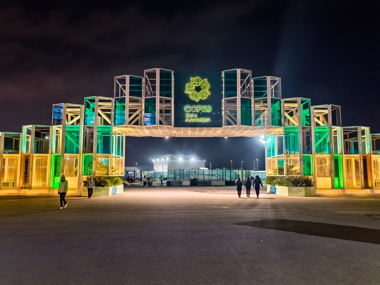
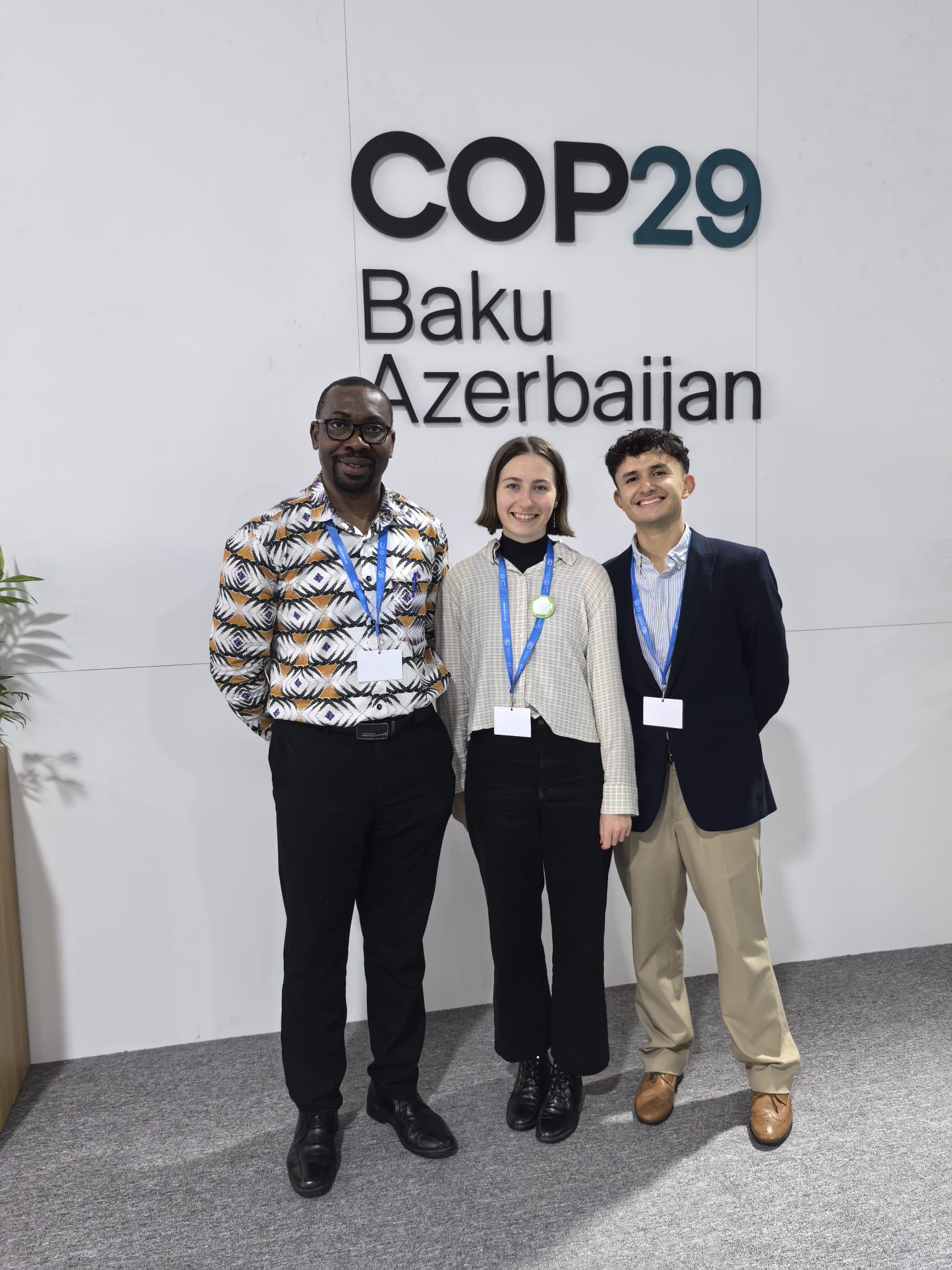
Picture 1, Entrance to COP29. Picture 2, Emmanuel Essah, Thea Stevens and Juan Garcia Valencia in COP29

Pre-COP 

What is COP29? 

COP29, the 29th Conference of the Parties, is the annual United Nations climate change conference and serves as the primary decision-making event under the United Nations Framework Convention on Climate Change (UNFCCC). Established by the treaty signed in 1992, COP brings together representatives from all UN member states and the European Union to address global climate challenges. This year, COP29 was held in November in Baku, Azerbaijan, drawing over 65,000 delegates from around the world, including diplomats, climate scientists, trade union leaders, and environmental activists. The event aims to negotiate effective strategies to combat the root causes of climate change. In essence, it’s the world’s largest and most significant gathering dedicated to climate action.

What were the expectations going into COP29?

Even before the summit began, COP29 was widely referred to as the “Finance COP” due to the prominence of one particular issue: climate finance. This term highlights the obligation of developed nations to provide financial resources to developing countries. These funds are intended to help nations build clean-energy systems, adapt to a warming world, and recover from disasters exacerbated by climate change. A significant focus of the negotiations and media coverage was the New Collective Quantified Goal (NCQG), a proposed climate finance target aimed at channelling resources to developing nations to combat climate change effectively.

However, discussions were also expected to extend beyond finance, addressing crucial topics such as Article 6 of the Paris Agreement, as well as strategies for adaptation and mitigation. We had the incredible opportunity to attend the second week of COP29—a pivotal stage of the process when ministers usually tackle the intricate details of agreements crafted in the first week, working to reach consensus. Heading into the conference, we anticipated hearing much more about the NCQG and its potential connections to other pressing climate issues.

Why did we apply to go?

“I decided to apply to attend COP29 due to the significance of geopolitical progress in ensuring that countries act in accordance with science. I think it is easy for us to forget the magnitude of what we study as meteorologists and climate scientists. To be able to follow how our scientific understanding shapes what actions are taken on a political scale feels important in order to put our work into context. I have also been following the progress of COPs for a long time – I was that geeky teenager in geography class who got a bit obsessed with the developments made there. So, on a more personal level, it also felt like a really exciting opportunity.” – Thea 

“My decision to apply for COP29 stemmed from a deep interest in the science-policy interface. As a PhD student researching monsoons and their variability with climate change, my work primarily involves analysing large datasets with the aim of crafting papers that can inform decision-making. While this scientific foundation is critical, I was eager to move beyond the confines of my computer screen and engage directly with the global climate community. This experience promised not only professional growth but also the chance to see firsthand how research and advocacy converge on the global stage so I knew I had to give it a go!” – Juan

What did we do in preparation? 

Having closely followed previous COPs and participated in COPCAS, we were familiar with the structure and nature of these conferences, which gave us a sense of what to expect. However, we knew that attending in person would be a completely different experience. In preparation, we undertook extensive training and courses. The Walker Institute’s help was invaluable, as they provided numerous opportunities to upskill and address our questions. They even arranged security training, given that we were heading to a politically sensitive region. Additionally, the IISD webinars were incredibly helpful in providing up-to-date insights on negotiation progress and key facts. Staying informed through these resources and keeping up with current news allowed us to approach the conference well-prepared and confident.

During COP 

What was the schedule like? 

The daily schedule at COP29 was intense. With only one week to make the most of the experience, our days were packed with meetings from 9:00AM – 6:00PM. We started each morning with the RINGO (Research and Independent Non-Governmental Organisations) meeting, which brought together members of the observer scientific community. These sessions provided a valuable space to discuss key themes and points of interest for the day, while also offering great networking opportunities.

The rest of the day was a whirlwind of press conferences, negotiations, and side events hosted by a wide range of organisations. Most events were open to all attendees, though some, particularly negotiations in the second week and high-profile press conferences (such as those featuring Antonio Guterres, Secretary-General of the UN!), were closed-door.

Another key aspect of our responsibilities was meeting twice daily with our team back at the Walker Institute. These sessions were a great chance to share our findings, report on the atmosphere on the ground, and receive valuable recommendations for upcoming events. More often than not, these check-ins also provided a much-needed energy and mood boost to keep us going through the busy days!

How did we decide on what to attend? 

Understanding the true scope of events and talks at COP took a while to get your head around. There is so much going on, and so much you could be going to it always felt like you were missing something. It was helpful to be able to think of the types of events you could go to into three different categories: the negotiations, the side events and the pavilion events. Each one of these had quite a different atmosphere, which was helpful to consider when deciding what to go to. 

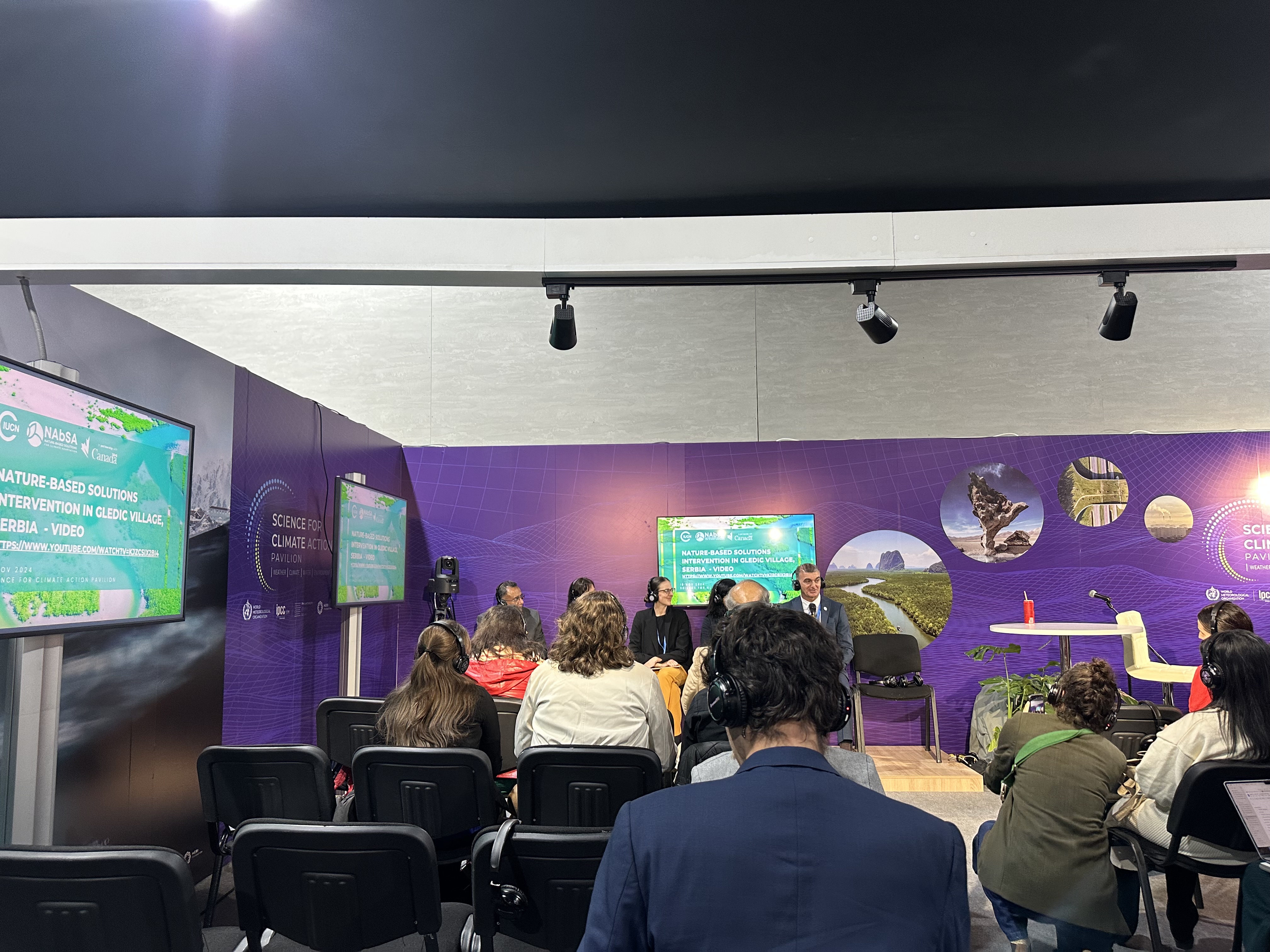
The pavilions were basically a full conference on their own, with every country and NGO having their own elaborately decorated area. Talks here were slightly more informal and there was a wide diversity of topics. If you wanted to get some information on a more specific topic and also have time to talk with the people presenting this was the place to be. 

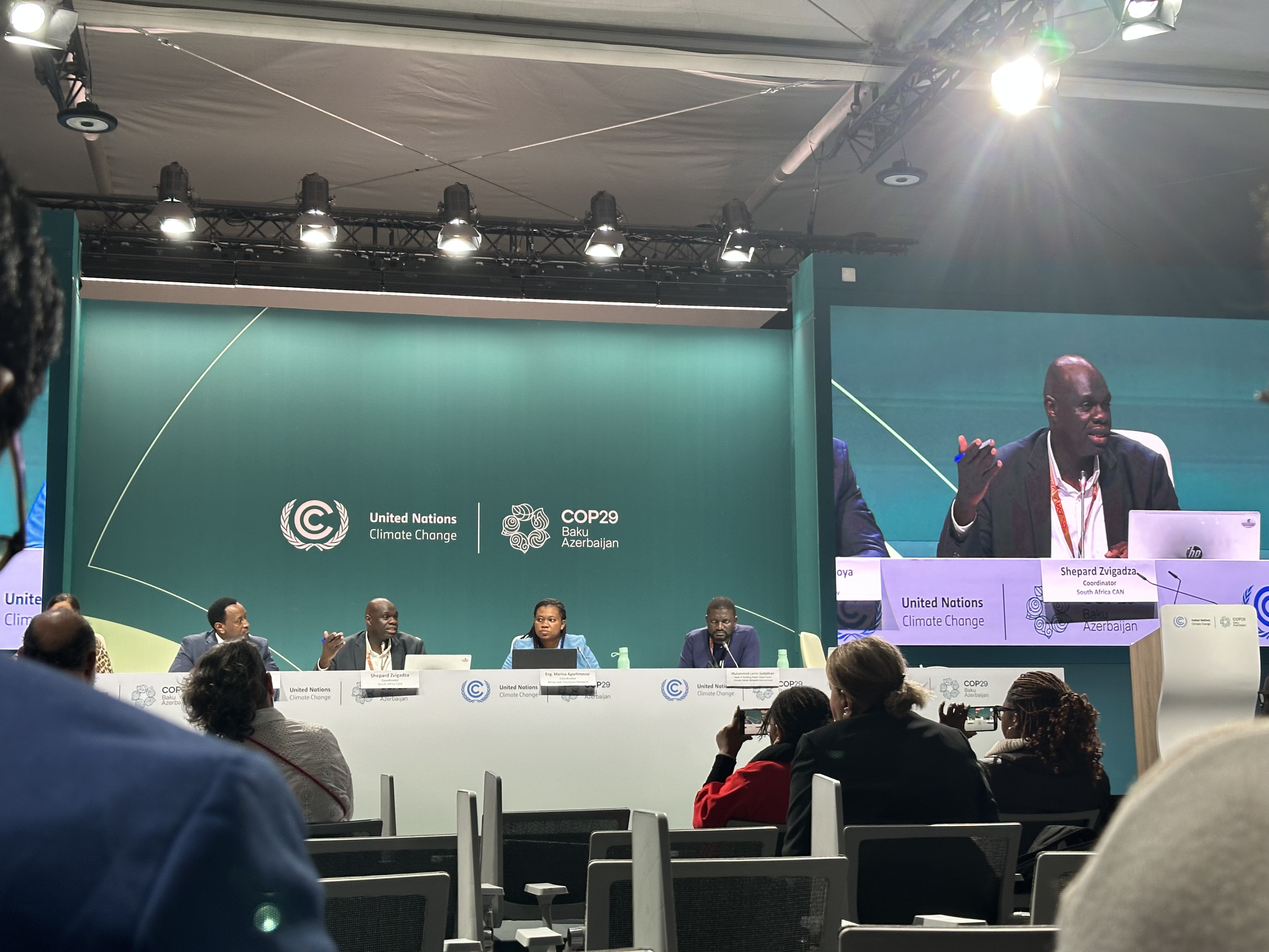
The side events were often more specific to the ongoing negotiations and included panel discussions and press conferences. These were often really exciting opportunities to get an update on the negotiations that we might not have been allowed to sit in on, and they often provided a more candid and emotive response to the developments. 

Lastly were the negotiations themselves. These were very slow and bureaucratic, but despite this, they were really fascinating to watch. It was what was going on in these negotiation rooms that really mattered to the outcome of COP! We had been given very good advice before we went to properly follow just one of the negotiation pieces so that you could understand how it was being shaped over time. However, as we attended the second week, the negotiations occurring behind closed doors increased more and more, and the agenda for these was constantly changing. We found it best to just jump on any opportunity there was to attend one of these as they became increasingly difficult to access. 

Having an overview of the different potential experiences in each of these parts of COP made it easier to asses what to go to and what might be interesting at any given time. 

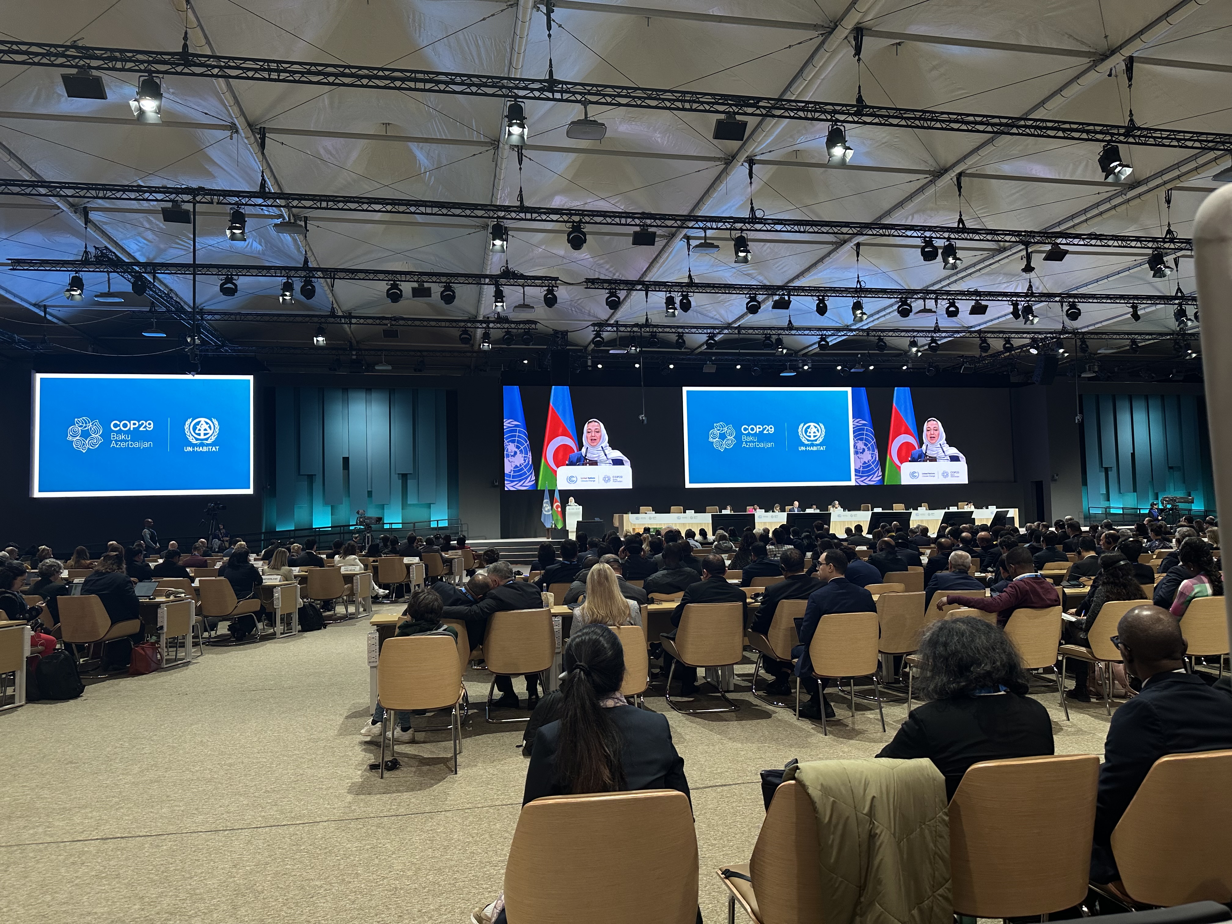
Picture 3, 4, and 5 show various events that happened in COP29, including a press conference, a science pavilion event and a plenary.

Who was someone interesting you met?

“While waiting in a queue to get into a negotiation, I met a delegate from an NGO based in South Africa. Through links to local religious groups, she helped guide communities to access climate-related financial aid. We discussed how amendments being made during different negotiations were having a direct impact on the accessibility of these funds. This provided a powerful reminder of how the negotiations had an impact on some of the most vulnerable communities not only in South Africa but all over the world. Having her watching and voicing opinions to negotiators between events provided a channel for these voices to be heard.” – Thea 

“Among the many incredible individuals I met, my interaction with two indigenous women from Chile left a profound impact. Their presentation on the consequences of lithium extraction in the Atacama Desert was both heartbreaking and inspiring. They spoke passionately about the devastating effects of privatized water and mineral resources, which have left their communities struggling with water scarcity and ecological exhaustion. Their unwavering determination to fight for their rights and protect their environment, despite significant challenges, was a powerful reminder of the human cost of unsustainable practices. Their story underscored the importance of amplifying marginalized voices in global climate discussions” – Juan

What is the role of the host country and how much influence do they have?

Hosting a COP entails significant responsibilities, including providing the facilities, security, and leadership required to ensure the summit’s success. In many ways, we were impressed by Azerbaijan’s efforts as the COP29 presidency. The facilities were well-prepared, and the transportation system was particularly noteworthy—clear, organised, and highly efficient, running seamlessly throughout the two weeks to help delegates commute to and from the conference centre with ease.

However, Azerbaijan’s selection as host sparked controversy from the moment it was announced at the end of COP28 in Dubai. One of the reasons was this it marked the third consecutive year that a petrostate was appointed to host the climate summit, raising concerns about potential conflicts of interest. This issue became a recurring theme throughout the conference, dominating discussions and even prompting high-profile criticisms. For example, Christiana Figueres, former UN climate chief, wrote an open letter during the first week, asserting that the COP process had become “no longer fit for purpose.”

By the second week, questions about the presidency’s ability to guide negotiations effectively were widespread. As the host country, Azerbaijan was expected to lead efforts to foster consensus among governments and non-Party stakeholders, particularly on critical issues like the NCQG and draft texts. Yet, progress was slow, and negotiations stretched into Saturday, further fuelling doubts about the presidency’s capacity to align its leadership with COP’s overarching goals.

Post-COP

What surprised you the most? 

“One of the most exciting and surprising things about COP was how accessible everything felt. As someone who wasn’t there for more than just to communicate what was happening to students at COPCAS, it felt really incredible that we were given access to the negotiations and all the plenary sessions. I obviously knew this was going to be the case before we went, but it was only really sitting when in on these events did I realise how unique of an opportunity this was.” – Thea

“One of the most striking aspects for me of attending last year’s COP was the incredible diversity of attendees, showcasing the universal impact of climate change and the essential need for broad representation in climate discussions. Among the most inspiring aspects was the strong presence of young people and activists, whose energy and commitment highlighted the vital role of the next generation in driving meaningful climate action” – Juan 

What do we think of the COP process? 

Going to COP and sitting in on the negotiations made the enormity of ambition and geopolitical complexity of bilateral agreements evident. Countries – with vastly different agendas and core beliefs – coming around a table trying to agree on something is an absurdly ambitious arrangement. Reducing fossil fuel consumption is unlike any another problem we face; their presence is pervasive in all of our lives. Fossil fuels are a bedrock of wealth and power in our global political economy. Despite alternative energies booming, and 2024 confirmed as the warmest year on record, this makes fossil fuels hard for the world to walk away from at the speed we need to do so. 

Whilst COP can be critiqued for being slow and disappointing, there remains hope in the vision of these bilateral negotiations. Given the increase in conflict and geopolitical instability these past few years, I left COP with an appreciation for the fact that there is still a negotiating table.

However, attending COP also brought to light how important it is to have ambitious domestic policies. COP will never really be the space where radical or big change will happen; this is instead the space where countries are all brought onto the same page. I think we left with more conviction that local politics and policies are where these larger changes need to happen.

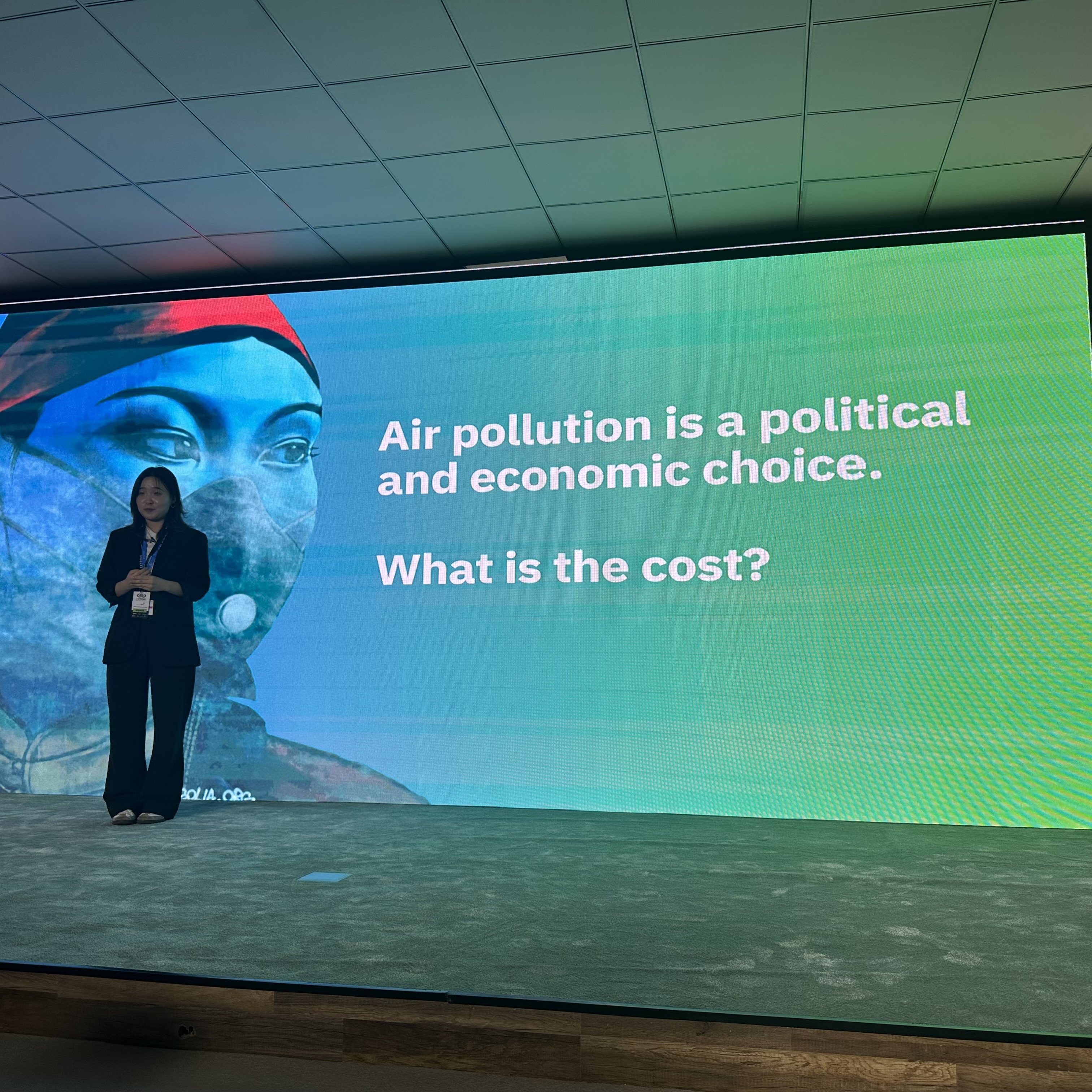
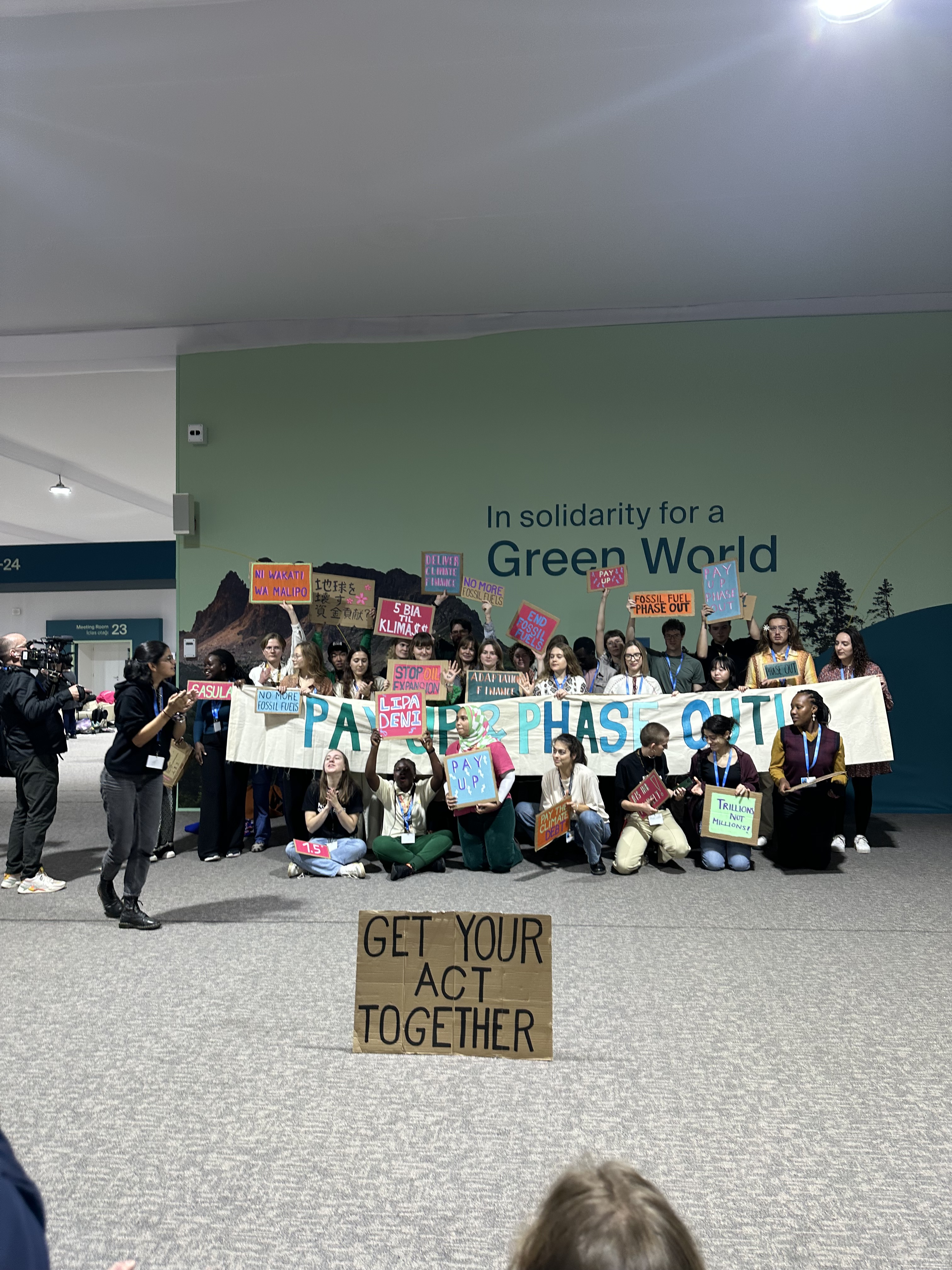
Picture 6, Powerful presentation by Enkhuun Byambadorji on Transforming Climate Narratives for Healthy. Picture 7, Organised protests by activists inside the Blue Zone.

Environments

What tips would you give to someone who is hoping to attend next year? 

  • Apply!! It’s an amazing opportunity both professionally and personally and it shouldn’t be missed. 
  • Wear comfortable yet formal attire. You will be walking around for most of the day but also meeting important and really cool people, so you definitely still want to look the part. 
  • Have business cards for networking 
  • Bring a power bank 
  • Practice your elevator pitch- in case you stumble across somebody interested in your research. 
  • Take lots of pictures!

Conclusion 

We wanted to end this blog by saying a massive thank you to the Walker Institute for their support in making this experience possible. Attending COP29 was a transformative journey that deepened our commitment to climate action and inspired us to continue advocating for a sustainable future.

Preparing for the assimilation of future ocean-current measurements

By Laura Risley

Ocean data assimilation (DA) is vital. Firstly, it is essential to improving forecasts of ocean variables. Not only that, the interaction between the ocean and atmosphere is key to numerical weather prediction (NWP) as coupled ocean-atmosphere DA schemes are used operationally.  

At present, observations of the ocean currents are not assimilated operationally. This is all set to change, as satellites are being proposed to measure these ocean currents directly. Unfortunately, the operational DA systems are not yet equipped to handle these observations due to some of the assumptions made about the velocities. In my work, we propose the use of alternative velocity variables to prepare for these future ocean current measurements. These will reduce the number of assumptions made about the velocities and is expected to improve the NWP forecasts.

What is DA? 

DA combines observations and a numerical model to give a best estimate of the state of our system – which we call our analysis. This will lead to a better forecast. To quote my lunchtime seminar ‘Everything is better with DA!’

Our model state usually comes from a prior estimate which we refer to as the background. A key component of data assimilation is that the errors present in both sets of data are taken into consideration. These uncertainties are represented by covariance matrices. 

I am particularly interested in variational data assimilation, which formulates the DA problem into a least squares problem. Within variational data assimilation the analysis is performed with a set of variables that differ from the original model variables, called the control variables. After the analysis is found in this new control space, there is a transformation back to the model space. What is the purpose of this transformation? The control variables are chosen such that they can be assumed approximately uncorrelated, reducing the complexity of the data assimilation problem.

Velocity variables in the ocean 

My work is focused on the treatment of the velocities in NEMOVAR. This is the data assimilation software used by the NEMO ocean model, used operationally at the Met Office and ECMWF. In NEMOVAR the velocities are transformed to their unbalanced components, and these are then used as control variables. The unbalanced components of the velocities are highly correlated, therefore contradicting the assumption made about control variables. This would result in suboptimal assimilation of future surface current measurements – therefore we seek alternative velocity control variables. 

The alternative velocity control variables we propose for NEMOVAR are unbalanced streamfunction and velocity potential. This would involve transforming the current control variables, the unbalanced velocities, to these alternative variables using Helmholtz Theorem. This splits a velocity field into its nondivergent (streamfunction) and irrotational (velocity potential) parts. These parts have been suggested by Daley (1993) as more suitable control variables than the velocities themselves. 

Numerical Implications of alternative variables 

We have performed the transformation to these proposed control variables using the shallow water equations (SWEs) on a 𝛽-plane. To do so we discretised the variables on the Arakawa-C grid. The traditional placement of streamfunction on this grid causes issues with the boundary conditions. Therefore, Li et al. (2006) proposed placing streamfunction in the centre of the grid, as shown in Figure 1. This circumvents the need to impose explicit boundary conditions on streamfunction. However, using this grid configuration leads to numerical issues when transforming from the unbalanced velocities to unbalanced streamfunction and velocity potential. We have analysed these theoretically and here we show some numerical results.

Figure 1: The left figure shows the traditional Arakawa-C configuration (Lynch (1989), Watterson (2001)) whereby streamfunction is in the corner of each grid cell. The right figure shows the Arakawa-C configuration proposed by Li et al. (2006) where streamfunction is in the centre of the grid cell. The green shaded region represents land. 

Issue 1: The checkerboard effect 

The transformation from the unbalanced velocities to unbalanced streamfunction and velocity potential involves averaging derivatives, due to the location of streamfunction in the grid cell. This process causes a checkerboard effect – whereby we have numerical noise entering the variable fields due to a loss of information. This is clear to see numerically using the SWEs. We use the shallow water model to generate a velocity field. This is transformed to its unbalanced components and then to unbalanced streamfunction and velocity potential. Using Helmholtz Theorem, the unbalanced velocities are reconstructed. Figure 2 shows the checkboard effect clearly in the velocity error.

Figure 2: The difference between the original ageostrophic velocity increments, calculated using the SWEs, and the reconstructed ageostrophic velocity increments. These are reconstructed using Helmholtz Theorem, from the ageostrophic streamfunction and velocity potential increments. On the left we have the zonal velocity increment error and on the right the meridional velocity increment error. 

Issue 2: Challenges in satisfying the Helmholtz Theorem 

Helmholtz theorem splits the velocity into its nondivergent and irrotational components. We discovered that although streamfunction should be nondivergent and velocity potential should be irrotational, this is not the case at the boundaries, as can be seen in figure 3. This implies the proposed control variables are able to influence each other on the boundary. This would lead to them being strongly coupled and therefore correlated near the boundaries. This directly conflicts the assumption made that our control variables are uncorrelated. 

Figure 3: Issues with Helmholtz Theorem near the boundaries. The left shows the divergence of the velocity field generated by streamfunction. The right shows the vorticity of the velocity field generated by velocity potential. 

Overall, in my work we propose the use of alternative velocity control variables in NEMOVAR, namely unbalanced streamfunction and velocity potential. The use of these variables however leads to several numerical issues that we have identified and discussed. A paper on this work is in preparation, where we discuss some of the potential solutions. Our next work will further this investigation to a more complex domain and assess our proposed control variables in assimilation experiments. 

References: 

Daley, R. (1993) Atmospheric data analysis. No. 2. Cambridge university press. 

Li, Z., Chao, Y. and McWilliams, J. C. (2006) Computation of the streamfunction and velocity potential for limited and irregular domains. Monthly weather review, 134, 3384–3394. 

Lynch, P. (1989) Partitioning the wind in a limited domain. Monthly weather review, 117, 1492–1500. 

Watterson, I. (2001) Decomposition of global ocean currents using a simple iterative method. Journal of Atmospheric and Oceanic Technology, 18, 691–703

Nature vs Nurture in Convective-Scale Ensemble Spread

By Adam Gainford

Quantifying the uncertainty of upcoming weather is now a common procedure thanks to the widespread use of ensemble forecasting. Unlike deterministic forecasts, which show only a single realisation of the upcoming weather, ensemble forecasts predict a range of possible scenarios given the current knowledge of the atmospheric state. This approach allows forecasters to estimate the likelihood of upcoming weather events by simply looking at the frequency of event occurrence within all ensemble members. Additionally, by sampling a greater range of events, this approach highlights plausible worst-case scenarios, which is of particular interest for forecasts of extreme weather. Understanding the realistic range of outcomes is crucial for forecasters to provide informed guidance, and helps us avoid the kind of costly and embarrassing mistakes that are commonly associated with the forecast of “The Great Storm of 1987”*.

To have trust that our ensembles are providing an appropriate range of outputs, we need some method of verifying ensemble spread. We do this by calculating the spread-skill relationship, which essentially just compares the difference between member values to the skill of the ensemble as a whole. If the spread-skill relationship is appropriate, spread and skill scores should be comparable when averaged over many forecasts. If the ensemble shows a tendency to produce larger spread scores than skill scores, there is too much spread and not enough confidence in the ensemble given its accuracy: i.e., the ensemble is overspread. Conversely, if spread scores are smaller than skill scores, the ensemble is too confident and is underspread. 

Figure 1: Postage stamp plots showing three-hourly precipitation accumulation valid for 2023-07-08 09Z at leadtime T+15 h. There is reasonable spread within both the frontal rain band effecting areas of SW England and Wales, and the convective features ahead of this front.

My PhD work has focussed on understanding the spread-skill relationship in convective-scale ensembles. Unlike medium range ensembles that are used to estimate the uncertainty of synoptic-scale weather at daily-to-weekly leadtimes, convective-scale ensembles quantify the uncertainty of smaller-scale weather at hourly-to-daily leadtimes. To do this, convective-scale ensembles must be run at higher resolutions than medium-range ensembles, with grid spacings smaller than 4 km. These higher resolutions allows the ensemble to explicitly represent convective storms, which has been repeatedly shown to produce more accurate forecasts compared coarser-resolution forecasts that must instead rely on convective parametrizations. However, running models at such high resolutions is too computationally expensive to be done over the entire Earth, so they are typically nested inside a lower-resolution “parent” ensemble which provides initial and boundary conditions. Despite this, researchers often report that convective-scale ensembles are underspread, and the range of outputs is too narrow given the ensemble skill. This is corroborated by operational forecasters, who report that the ensemble members often stay too close to the unperturbed control member. 

To provide the necessary context for understanding the underspread problem, many studies have examined the different sources and behaviours of spread within convective-scale ensembles. In general, spread can be produced through three different mechanisms: firstly, through differences in each member’s initial conditions; secondly, through differences in the lateral boundary conditions provided to each member; and thirdly, through the different internal processes used to evolve the state. This last source is really the combination of many different model-specific factors (e.g., stochastic physics schemes, random parameter schemes etc.), but for our purposes this represents the ways in which the convective-scale ensemble produces its own spread. This contrasts with the other two sources of spread, which are directly linked to the spread of the parent ensemble.  

The evolution of each of these three spread sources is shown in Fig. 2. At the start of a forecast, the ensemble spread is entirely dictated by differences in the initial conditions provided to each ensemble member. As we integrate forward in time, though, this initial information is removed from the domain by the prevailing winds and replaced by information arriving through the boundaries. At the same time, internal model processes start spinning up additional detail within each ensemble member. For a UK-sized domain, it takes roughly 12 hours for the initial information to have fully left the domain, though this is of course highly dependent on the strength of the prevailing winds. After this time, spread in the ensemble is partitioned between internal processes and boundary condition differences.  

Figure 2: Attribution of spread within a convective-scale ensemble by leadtime. 

While the exact partitioning in this schematic shouldn’t be taken too literally, it does highlight the important role that the parent ensemble plays in determining spread in the child ensemble. Most studies which try to improve spread target the child ensemble itself, but this schematic shows that these improvements may have quite a limited impact. After all, if the spread of information arriving from the parent ensemble is not sufficient, this may mask or even overwhelm any improvements introduced to the child ensemble.  

However, there are situations where we might expect internal processes to show a more dominant spread contribution. Forecasts of convective storms, for instance, typically show larger spread than forecasts of other types of weather, and are driven more by local processes than larger-scale, external factors.

This is where our “nature” and “nurture” analogy becomes relevant. Given the similarities of this relationship to the common parent-child theory in behavioural psychology, we thought it would be a fun and useful gimmick to also use this terminology here. So, in the “nature” scenario, each child member shows large similarity to the corresponding parent member, which is due to the dominating influence of genetics (initial and boundary conditions). Conversely, in the “nurture” scenario, spread in the child ensemble is produced more by its response to the environment (internal processes), and as such, we see larger differences between each parent-child pair.  

While the nature and nurture attribution is well understood for most variables, few studies have examined the parent-child relationship for precipitation patterns, which are an important output for guidance production and require the use of neighbourhood-based metrics for robust evaluation. Given that this is already quite a long post, I won’t go into too much detail of our results looking at nature vs nurture for precipitation patterns. Instead, I will give a quick summary of what we found: 

  • Nurture provides a larger than average influence on the spread in two situations: during short leadtimes**, and when forecasting convective events driven by continental plume setups. 
  • In the nurture scenarios, spread is consistently larger in the child ensemble than the parent ensemble. 
  • In contrast to the nurture scenarios, nature provides larger than average spread at medium-to-long leadtimes and under mobile regimes, which is consistent with the boundary arguments mentioned previously. 
  • Spread is very similar between the child and parent ensembles in the nurture scenarios.  

If you would like to read more about this work, we will be submitting a draft to QJRMS very soon.  

To conclude, if we want to improve the spread of precipitation patterns in convective-scale ensembles, we should direct more attention to the role of the driving ensemble. It is clear that the exact nesting configuration used has a strong impact on the quality of the spread. This factor is especially important to consider given recent experiments with hectometric-scale ensembles which are themselves nested within convective-scale ensembles. With multiple layers of nesting, the coupling between each ensemble layer is likely to be complex. Our study provides the foundation for investigating these complex interactions in more detail. 

* This storm was actually well forecast by the Met Office. The infamous Michael Fish weather update in which he said there was no hurricane on the way was referring to a different system which indeed did not impact the UK. Nevertheless, this remains a good example of the importance of accurately predicting (and communicating) extreme weather events.  

** While this appears to be inconsistent with Fig. 2, the ensemble we used does not solely take initial conditions from the driving ensemble. Instead, the ensemble uses a separate, high-resolution data assimilation scheme to the parent ensemble. Each ensemble is produced in a way which makes the influence of the data assimilation more influential to the spread than the initial condition perturbations. 

The 5th ICTP Summer School on Modelling of Climate Dynamics: Convection and Clouds, and Conference on Convective Organisation (WCO4)

By Juan Garcia Valencia

In the tropics, organised convective systems provide the majority of precipitation and are often responsible for extreme events. To understand these systems, researchers now use kilometre-resolution (k-scale) global and regional convection-permitting models, along with the latest satellite observations. Machine learning tools have also emerged as important supplements to our dynamical and thermodynamic understanding.

It’s crucial to understand these tools to address key questions such as:

  • How do deep and shallow convection organise in k-scale models?
  • Can energy budgets help explain their precipitation biases?
  • What are the recent advances in convective parameterisation?

These questions were the focus of the “5th Summer School on Theory, Mechanisms and Hierarchical Modelling of Climate Dynamics: Convection and Clouds,” which I had the privilege of attending from the 1st–19th of July 2024 at the International Centre for Theoretical Physics (ICTP) in Trieste, Italy.

Picture 1 and 2. First lecture and campus. 

The program offered a mix of introductory and advanced lectures, hands-on data analysis through participant projects, and the chance to get involved in the “4th Workshop on Convective Organisation and Precipitation Extremes (WCO4).” The opportunity to attend arose because two of my supervisors, Chris Holloway and Lorenzo Tomassini, presented their work at the conference and taught some of the lectures in the course. As a PhD student researching monsoons using kilometre-scale simulations, I also felt like I had to attend! 

The three-week schedule was intense, with most days running from 9 AM to 6 PM (thankfully with plenty of coffee breaks and a long lunch). A typical day began with lectures from leading experts like Simona Bordoni, Robert Pincus, and Courtney Schumacher. Topics ranged from convection and radiation to RCE, stochastic parameterisation, and observations. Afternoons were usually dedicated to computer lab sessions or group project work.

Picture 3. Attendees of the summer school. 

The second week centred on the WCO4 conference, covering topics from convective self-aggregation in idealized experiments to precipitation extremes associated with organized convection and optimizing our use of observational data. Students had the opportunity to present posters on their research—an incredibly valuable experience for me as I received loads of useful feedback about my ideas and goals. This was also my first time presenting research at an international event, so it was great to show what I’ve been working on in front of all the attendees and meet so many people genuinely interested in my work.

The final week focused on hands-on projects. In groups of 4–5, we analysed numerical model data and presented our results to everyone. My group examined how precipitation extremes change in a warming world using NextGEMS data, but every group had different topics that they had chosen according to their interest and expertise. Many of the tasks and analyses we did were similar to my first-year work, so I left with a plenty of new ideas for my research!

Picture 4. End of group project presentation and poster presentation. 

Being an international centre, the school and conference brought together staff and students from all corners of the globe—one of my favourite aspects of the course. Despite knowing no one beforehand, I quickly got to know other PhDs and post-docs from various institutions, all working on projects similar to mine. I felt at ease in this new environment, making friends and meeting potential future colleagues!

Another fantastic aspect of this summer school was its stunning location on Italy’s sunny, warm northern Adriatic coast. After each day’s activities, we were free to spend our evenings as we pleased. This was the perfect opportunity to relax by the sea, swim, and explore Trieste’s picturesque town centre. More often than not, we’d venture into town for pizza and, of course, gelato!