By Adam Gainford
Quantifying the uncertainty of upcoming weather is now a common procedure thanks to the widespread use of ensemble forecasting. Unlike deterministic forecasts, which show only a single realisation of the upcoming weather, ensemble forecasts predict a range of possible scenarios given the current knowledge of the atmospheric state. This approach allows forecasters to estimate the likelihood of upcoming weather events by simply looking at the frequency of event occurrence within all ensemble members. Additionally, by sampling a greater range of events, this approach highlights plausible worst-case scenarios, which is of particular interest for forecasts of extreme weather. Understanding the realistic range of outcomes is crucial for forecasters to provide informed guidance, and helps us avoid the kind of costly and embarrassing mistakes that are commonly associated with the forecast of “The Great Storm of 1987”*.
To have trust that our ensembles are providing an appropriate range of outputs, we need some method of verifying ensemble spread. We do this by calculating the spread-skill relationship, which essentially just compares the difference between member values to the skill of the ensemble as a whole. If the spread-skill relationship is appropriate, spread and skill scores should be comparable when averaged over many forecasts. If the ensemble shows a tendency to produce larger spread scores than skill scores, there is too much spread and not enough confidence in the ensemble given its accuracy: i.e., the ensemble is overspread. Conversely, if spread scores are smaller than skill scores, the ensemble is too confident and is underspread.
My PhD work has focussed on understanding the spread-skill relationship in convective-scale ensembles. Unlike medium range ensembles that are used to estimate the uncertainty of synoptic-scale weather at daily-to-weekly leadtimes, convective-scale ensembles quantify the uncertainty of smaller-scale weather at hourly-to-daily leadtimes. To do this, convective-scale ensembles must be run at higher resolutions than medium-range ensembles, with grid spacings smaller than 4 km. These higher resolutions allows the ensemble to explicitly represent convective storms, which has been repeatedly shown to produce more accurate forecasts compared coarser-resolution forecasts that must instead rely on convective parametrizations. However, running models at such high resolutions is too computationally expensive to be done over the entire Earth, so they are typically nested inside a lower-resolution “parent” ensemble which provides initial and boundary conditions. Despite this, researchers often report that convective-scale ensembles are underspread, and the range of outputs is too narrow given the ensemble skill. This is corroborated by operational forecasters, who report that the ensemble members often stay too close to the unperturbed control member.
To provide the necessary context for understanding the underspread problem, many studies have examined the different sources and behaviours of spread within convective-scale ensembles. In general, spread can be produced through three different mechanisms: firstly, through differences in each member’s initial conditions; secondly, through differences in the lateral boundary conditions provided to each member; and thirdly, through the different internal processes used to evolve the state. This last source is really the combination of many different model-specific factors (e.g., stochastic physics schemes, random parameter schemes etc.), but for our purposes this represents the ways in which the convective-scale ensemble produces its own spread. This contrasts with the other two sources of spread, which are directly linked to the spread of the parent ensemble.
The evolution of each of these three spread sources is shown in Fig. 2. At the start of a forecast, the ensemble spread is entirely dictated by differences in the initial conditions provided to each ensemble member. As we integrate forward in time, though, this initial information is removed from the domain by the prevailing winds and replaced by information arriving through the boundaries. At the same time, internal model processes start spinning up additional detail within each ensemble member. For a UK-sized domain, it takes roughly 12 hours for the initial information to have fully left the domain, though this is of course highly dependent on the strength of the prevailing winds. After this time, spread in the ensemble is partitioned between internal processes and boundary condition differences.
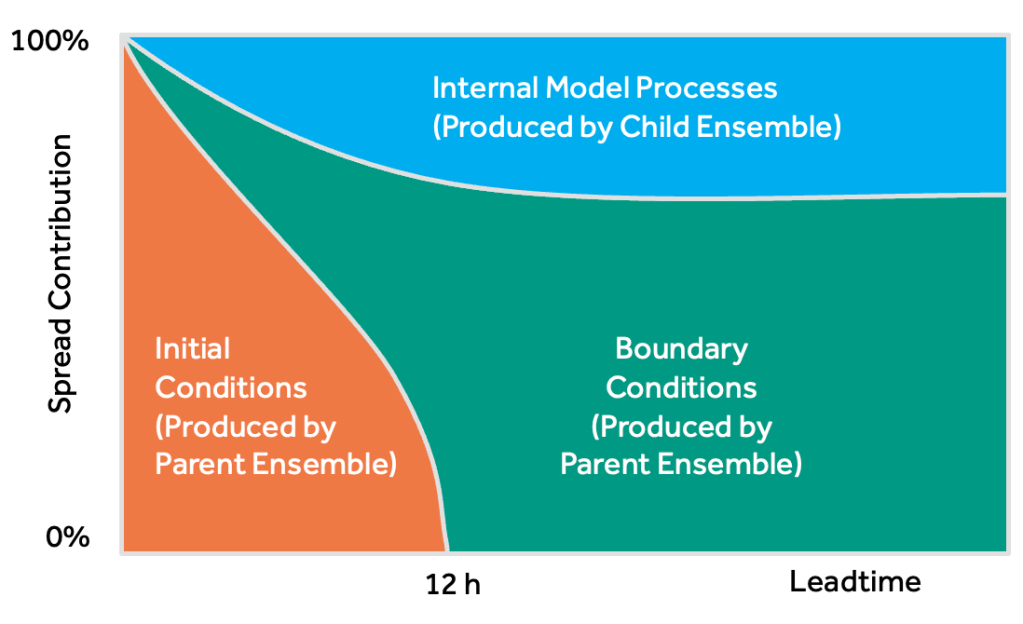
While the exact partitioning in this schematic shouldn’t be taken too literally, it does highlight the important role that the parent ensemble plays in determining spread in the child ensemble. Most studies which try to improve spread target the child ensemble itself, but this schematic shows that these improvements may have quite a limited impact. After all, if the spread of information arriving from the parent ensemble is not sufficient, this may mask or even overwhelm any improvements introduced to the child ensemble.
However, there are situations where we might expect internal processes to show a more dominant spread contribution. Forecasts of convective storms, for instance, typically show larger spread than forecasts of other types of weather, and are driven more by local processes than larger-scale, external factors.
This is where our “nature” and “nurture” analogy becomes relevant. Given the similarities of this relationship to the common parent-child theory in behavioural psychology, we thought it would be a fun and useful gimmick to also use this terminology here. So, in the “nature” scenario, each child member shows large similarity to the corresponding parent member, which is due to the dominating influence of genetics (initial and boundary conditions). Conversely, in the “nurture” scenario, spread in the child ensemble is produced more by its response to the environment (internal processes), and as such, we see larger differences between each parent-child pair.
While the nature and nurture attribution is well understood for most variables, few studies have examined the parent-child relationship for precipitation patterns, which are an important output for guidance production and require the use of neighbourhood-based metrics for robust evaluation. Given that this is already quite a long post, I won’t go into too much detail of our results looking at nature vs nurture for precipitation patterns. Instead, I will give a quick summary of what we found:
- Nurture provides a larger than average influence on the spread in two situations: during short leadtimes**, and when forecasting convective events driven by continental plume setups.
- In the nurture scenarios, spread is consistently larger in the child ensemble than the parent ensemble.
- In contrast to the nurture scenarios, nature provides larger than average spread at medium-to-long leadtimes and under mobile regimes, which is consistent with the boundary arguments mentioned previously.
- Spread is very similar between the child and parent ensembles in the nurture scenarios.
If you would like to read more about this work, we will be submitting a draft to QJRMS very soon.
To conclude, if we want to improve the spread of precipitation patterns in convective-scale ensembles, we should direct more attention to the role of the driving ensemble. It is clear that the exact nesting configuration used has a strong impact on the quality of the spread. This factor is especially important to consider given recent experiments with hectometric-scale ensembles which are themselves nested within convective-scale ensembles. With multiple layers of nesting, the coupling between each ensemble layer is likely to be complex. Our study provides the foundation for investigating these complex interactions in more detail.
* This storm was actually well forecast by the Met Office. The infamous Michael Fish weather update in which he said there was no hurricane on the way was referring to a different system which indeed did not impact the UK. Nevertheless, this remains a good example of the importance of accurately predicting (and communicating) extreme weather events.
** While this appears to be inconsistent with Fig. 2, the ensemble we used does not solely take initial conditions from the driving ensemble. Instead, the ensemble uses a separate, high-resolution data assimilation scheme to the parent ensemble. Each ensemble is produced in a way which makes the influence of the data assimilation more influential to the spread than the initial condition perturbations.


 ) at each time step in each group, and compare these fields between groups to see if I can find a source of forecast error.