Climate model systematic biases in the Maritime Continent

Email: y.y.toh@pgr.reading.ac.uk

The Maritime Continent commonly refers to the groups of islands of Indonesia, Borneo, New Guinea and the surrounding seas in the literature. My study area covers the Maritime Continent domain from 20°S to 20°N and 80°E to 160°E as shown in Figure 1. This includes Indonesia, Malaysia, Brunei, Singapore, Philippines, Papua New Guinea, Solomon islands, northern Australia and parts of mainland Southeast Asia including Thailand, Laos, Cambodia, Vietnam and Myanmar.

subsetF1
Figure 1: JJA precipitation (mm/day) and 850 hPa wind (m s−1) for (a) GPCP and ERA-interim, (b) MMM biases and (c)–(j) AMIP biases for 1979–2008 over the Maritime Continent region (20°S–20ºN, 80°E–160ºE). Third panel shows the Maritime Continent domain and land-sea mask

The ability of climate model to simulate the mean climate and climate variability over the Maritime Continent remains a modelling challenge (Jourdain et al. 2013). Our study examines the fidelity of Coupled Model Intercomparison Project phase 5 (CMIP5) models at simulating mean climate over the Maritime Continent. We find that there is a considerable spread in the performance of the Atmospheric Model Intercomparison Project (AMIP) models in reproducing the seasonal mean climate and annual cycle over the Maritime Continent region. The multi-model mean (MMM) (Figure 1b) JJA precipitation and 850hPa wind biases with respect to observations (Figure 1a) are small compared to individual model biases (Figure 1c-j) over the Maritime Continent. Figure 1 shows only a subset of Fig. 2 from Toh et al. (2017), for the full figure and paper please click here.

We also investigate the model characteristics that may be potential sources of bias. We find that AMIP model performance is largely unrelated to model horizontal resolution. Instead, a model’s local Maritime Continent biases are somewhat related to its biases in the local Hadley circulation and global monsoon.

cluster2
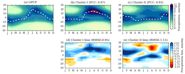
Figure 2: Latitude-time plot of precipitation zonally averaged between 80°E and 160°E for (a) GPCP, (b) Cluster I and (c) Cluster II. White dashed line shows the position of the maximum precipitation each month. Precipitation biases with respect to GPCP for (d) Cluster I and (e) Cluster II.

To characterize model systematic biases in the AMIP runs and determine if these biases are related to common factors elsewhere in the tropics, we performed cluster analysis on Maritime Continent annual cycle precipitation. Our analysis resulted in two distinct clusters. Cluster I (Figure 2b,d) is able to reproduce the observed seasonal migration of Maritime Continent precipitation, but it overestimates the precipitation, especially during the JJA and SON seasons. Cluster II (Figure 2c,e) simulate weaker seasonal migration of Intertropical Convergence Zone (ITCZ) than observed, and the maximum rainfall position stays closer to the equator throughout the year. Tropics-wide properties of clusters also demonstrate a connection between errors at regional scale of the Maritime Continent and errors at large scale circulation and global monsoon.

On the other hand, comparison with coupled models showed that air-sea coupling yielded complex impacts on Maritime Continent precipitation biases. One of the outstanding problems in the coupled CMIP5 models is the sea surface temperature (SST) biases in tropical ocean basins. Our study highlighted central Pacific and western Indian Oceans as the key regions which exhibit the most surface temperature correlation with Maritime Continent mean state precipitation in the coupled CMIP5 models. Future work will investigate the impact of SST perturbations in these two regions on Maritime Continent precipitation using Atmospheric General Circulation Model (AGCM) sensitivity experiments.


References:

Jourdain N.C., Gupta A.S., Taschetto A.S., Ummenhofer C.C., Moise A.F., Ashok K. (2013) The Indo-Australian monsoon and its relationship to ENSO and IOD in reanalysis data and the CMIP3/CMIP5 simulations. Climate Dynamics. 41(11–12):3073–3102

Toh, Y.Y., Turner, A.G., Johnson, S.J., & Holloway, C.E. (2017). Maritime Continent seasonal climate biases in AMIP experiments of the CMIP5 multimodel ensemble. Climate Dynamics. doi: 10.1007/s00382-017-3641-x

Why become a Royal Meteorological Society Student member?

This week the Royal Meteorological Society (RMetS) published their strategic plan for the period of 2018 to 2020, and here at Social Metwork HQ we thought it would be a splendid idea to reflect on the benefits of being a student member of the Royal Meteorological Society.

An important benefit in my opinion is that when becoming a member of RMetS you join a well-established community who hold enthusiasm about the weather and climate at its core. Members come from all corners of the world and at different stages of their career spanning the entire range: from the amateur weather enthusiasts to professionals.  nicole-kuhn-450747As a student, being an RMetS member can lead to conversations that could develop your career and bring unexpected opportunities. This has been greatly enhanced with the RMetS mentoring scheme.

RMetS host many different types of meetings, including annual conferences, meetings hosted by regional centres, and national meetings. Additional gatherings are held by special interest groups, ranging from Weather Arts & Music to Dynamical Problems. Meetings on a regional and national scale provide a platform for discussion and learning amongst those in the field. DEhXj9AXkAARyMM.jpg largeFor a student, the highlight in the RMetS calendar is the annual student conference. Every year, sixty to eighty students come together to present their work and develop professional relationships that continue for years to come. This year’s conference is hosted at the University of York on the 5th and 6th July 2018 (more information). After two student conferences under my belt (see previous blog post), I would highly recommend any early career research scientist attending this event. It serves as a platform to share their own work in a friendly atmosphere and be inspired by the wider student community.

nasa-63030Other benefits to becoming an RMetS student member include eligibility to the Legacies Fund, grants and fellowships, and receiving a monthly copy of Weather magazine. Most importantly though, through becoming a RMetS member you support a professional society who are committed to increasing awareness of the importance of weather and climate in policy and decision-making. Alongside this week’s publication of RMetS’ strategic plan, both the Met Office and NASA have published press releases stating that 2017 was the warmest year on record without El Niño. The atmosphere and oceans of our planet are changing at unprecedented rates: rising sea levels, reductions in Arctic sea-ice, and an increased frequency of extreme weather events to name but a few climate change impacts. Becoming an RMetS student member does not only benefit your career and knowledge, but also supports a society that is committed to promoting and raising awareness of weather and climate science.

VMSG and COMET 2018 (or a Tale of Two Conferences)

The Volcanic and Magmatic Studies Group (VMSG) held a conference from the 3-6th of January in Leeds. The Centre for Observation and Modelling of Earthquakes, Volcanoes and Tectonics (COMET) held a student conference from 8-9th January in Cambridge. It was a conference double-whammy about all things volcanic – heaven!

VMSG is a joint special interest group of the Mineralogical Society of Great Britain and Ireland and the Geological Society of London. The VMSG conference is a fairly small affair, with about 200 in attendance, and it brings together research in geochemistry, seismology, volcanology and related fields. Because of its size, it’s a nice informal space where there is a focus on students presenting their work to the VMSG community, but anyone is free to present their research.

Talks ranged from how tiny fossils, called diatoms, became trapped in a pyroclastic density current, to modelling of lava domes, to how local people interact with the volcano they live on at Masaya, to every aspect of volcanology you can think of. The final talk was definitely a highlight – with everyone in 3D glasses to look at volcanic plumes across Russia, it really brought the satellite images to life (and we got to keep the glasses).

90 posters on a variety of topics were presented, the majority of which were by students (I was one of them). There was of course an obligatory dinner and disco to round off the second day of talks, and a great chance to network with other people from VMSG.

For the best poster title of the conference, you need look no further than this gem.

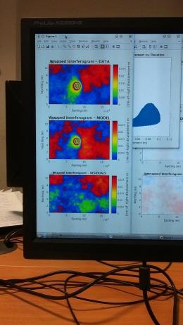
The conference also provides workshops on different aspects of research, with sessions on writing papers, diffusion modelling and InSAR to name a few. These were hosted on the 6th at the University of Leeds Environment and Earth Sciences Department, and comprised a full day of talks and labs so you could get to grips with the techniques you were being shown. I attended the InSAR workshop, which gave a good introduction to the topic of comparing two satellite images and seeing where the ground had moved. There was also a session on deformation modelling in the afternoon and playing with bits of code.

26771981_1615887968434336_143604950_o
An afternoon of modelling InSAR deformations and code – hill-arity ensued.

Then it was onto the second leg of the conferences, which took the action to Cambridge, where students that are part of COMET met up to discuss work and attend talks from 8-9th January.

26732711_1615887681767698_951066323_o
Gneiss weather in Cambridge!

COMET is a National Environment Research Council Centre of Excellence, it comprises a group of researchers that uses remote and ground sensed data and models to study earthquakes and volcanoes. They also work with the British Geological Survey and the European Space Agency, and fund PhD projects in related fields.

The meet-up of students comprised two days of talks from students, with some keynote speakers who had been past members of COMET that had gone on to careers outside of academia. The talks from second and third years included: remote sensing and InSAR being used to examine tectonic strain in the East African Rift Valley and slip (movement) rates along faults in Tibet, modelling how gas bubbles in magma change the more crystals you add to the magma, and using cosmogenic isotopes to work out slip rates on a fault in Italy.

26695576_1615887065101093_724648553_o
The Department had cabinets and cabinets of samples that rocked.

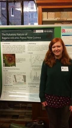
First years are also given the chance to give a talk lasting 5 minutes, so I filled people in on what I’d been up to in the past four months – lots of data collection! My project will be using satellite data to look at the varied eruption behaviour of Bagana volcano in Papua New Guinea, with a view to modelling this behaviour to better understand what causes it. Bagana has a tendency to send out thick lava flows in long pulses and let out lots of gas, and occasionally then violently erupt and let out lots of ash and hot pyroclastic density currents. But it is very understudied, as it is so remote – so there’s lots still to be learnt about it!

26736005_1616717381684728_2011570642_o
Me with my poster (I’ve run out of geology puns).

The meet-up also included a fancy meal in Pembroke College’s Old Library, with candles and it felt a bit like being at Hogwarts! Then it was back to Reading, thoroughly worn out, but with lots of ideas and many useful contacts – VMSG2019 is in St. Andrews and I can’t wait.

Deficiencies in climate model simulations of the seasonal rains in Africa

Email: c.m.dunning@pgr.reading.ac.uk

‘When is the wet season in Britain?’ a new student from Botswana asked me once. ‘Errrr, January-December?’ I replied flippantly. But in Botswana, and across much of Africa they experience one or two well-defined wet seasons per year, when the majority of the annual rainfall occurs. The timing and length of this wet season(s) is of significant societal importance; it replenishes water supplies used for drinking and other domestic purposes, affects the agricultural growing seasons and impacts the lifecycle of a number of vectors associated with the transmission of diseases such as malaria and dengue fever. Delays in the onset, or even failure of the wet season, can lead to reduced yields and potential food insecurity.

Future changes in climate will not be felt solely through changes in mean climate; projected shifts in atmospheric circulation patterns will also alter seasonality. Africa is acutely vulnerable to the effects of climate change so understanding future changes in the seasonal cycle of African precipitation is of utmost importance in establishing appropriate adaptation strategies. In order to produce reliable projections of seasonality, we require models to contain an accurate representation of current seasonality.

In our recent study we use a novel method to diagnose progression of the rainy seasons across continental Africa and identify important deficiencies in the climate simulations (a previous blog post and paper describes this method).

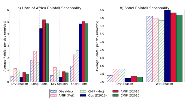
Firstly, when we use the method of Dunning et al. (2016) to identify the wet seasons in satellite-based precipitation estimates, atmosphere-only and coupled climate model simulations we find that the rainy seasons are differentiated more clearly from the dry seasons (shown by larger differences in the average rainfall per rainy day; Figure 1) than when fixed meteorological seasons (OND, MAM etc) are used, as this method accounts for interannual variability in seasonal timing and model timing biases.

figure_1anew

Figure 1. Average rainfall rate (mm day−1) during the wet/dry seasons over the Horn of Africa (a) and the Sahel (b) when defined using meteorological seasons (dashed bars) and dynamically varying seasons (Dunning et al. 2016, solid). See Figure 2 for a map of the regions.

Overall, climate model simulations capture the gross seasonal cycle of African precipitation on a continental scale, and seasonal timing exhibits good agreement with observations, however deficiencies manifest over key regions (Figure 2). The Horn of Africa (Somalia, southern Ethiopia, Kenya) experiences two wet seasons per year; the ‘long rains’ during March-May and the ‘short rains’ during October-November.  Whilst the simulations capture two wet seasons per year, they exhibit significant timing biases, with the long rains around 3 weeks late and the short rains nearly 4 weeks too long on average (Figure 2). Accounting for these biases may be crucial in interpreting the contrasting trend of observed declining rainfall during the ‘long rains’ in recent years and model projections of increasing ‘long rains’ rainfall in the future.

figure_4_regions_withbars_newlegend

Figure 2: Multi-model mean onset (open circles) and cessation (filled squares) for observations, atmosphere-only (AMIP) and coupled (CMIP) over selected regions (b). Shaded bars indicate the period of the wet season. For SWAC the mean annual regime onset/cessation in coupled simulations is plotted, along with mean onset/cessation for MIROC4h and BCC-CSM1-1-M (coupled simulations).

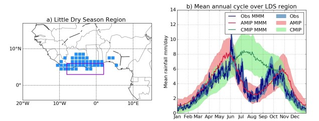
The most notable bias affects the southern coastline of West Africa, a region of complex meteorology with growing population and declining air quality. This region experiences the first wet season from April-June and the second wet season from mid-September-October, separated by the ‘Little Dry Season’ (LDS) in July-August. The LDS can be useful for weeding and spraying crops with pesticides between the two wet seasons, but can adversely affect crop yields if it is too long or pronounced. We find that simulations produce an unrealistic single summer wet season, with no mid-summer break in the rains and this is linked with biases in ocean temperature patterns. Given that climate simulations cannot capture the current seasonality, future projections for this region should be treated with caution.

Tweet_Fig5

Figure 3: a) Location of the region that experiences the Little Dry Season (LDS; blue dots) and the SST region of interest (pink box). b) Mean annual cycle of rainfall in observations, atmosphere-only and coupled simulations over LDS region.

This work highlights important deficiencies in the representation of the seasonal cycle of rainfall by climate simulations with implications for the reliability of future climate projections and associated impact assessments, including water availability for hydropower generation, the length of the malaria transmission season and future crop yields.

The full paper can be found here:

Dunning, C.M., Allan, R.P. and Black, E. (2017) Identification of deficiencies in seasonal rainfall simulated by CMIP5 climate models, Environmental Research Letters, 12(11), 114001, doi:10.1088/1748-9326/aa869e


A week at COP23

From the 6th -17th of November the UNFCCC’s (United Nation Framework Convention on Climate Change) annual meeting or “Conference of the Parties” – COP took place. This year was COP23 and was hosted by Bonn in the UN’s world conference centre with Fiji taking the presidency.

IMG_20171106_123155780

Heading into the Bonn Zone on the first day of the COP. The Bonn Zone was the part of the conference for NGO stands and side events.

As part of the Walker Institutes Climate Action Studio another SCENARIO PhD and I attended the first week of the COP while students back in Reading participated remotely via the UNFCCC’s YouTube channel and through interviews with other participants of the COP.

There are many different components to the COP, it is primarily the meeting of a number of different international Climate agreements with lots of work currently being done on the implementation on the Paris Agreement. However it is also a space where many different civil society groups doing work connected to or impacted by climate change come together, to make connections with other NGOs as well as governments. This is done in an official capacity within the “exhibition zone” of the conference and with a vast array of side events taking place throughout the two weeks. Outside of these official events there are also many demonstrations both inside and outside of the conference space.

Demonstrations in the Bonn Zone

As an observer I was able to watch some of the official negotiations. On the Wednesday I attended the SBSTA (Subsidiary Body for Scientific and Technological Advice) informal consultation on research and systematic observations. It was an illuminating experience to see the negotiation process in action. At times it was frustrating to see how picky it feels like the negotiation teams can be, however over the week I did have a newfound appreciation for the complexity of the issues that are having to be resolved. This meeting was based on writing a short summary of the IPCC report and other scientific reports used by the COP, and so was less politically charged than a lot of the other meetings. However this didn’t stop an unexpected amount of debate over whether to include examples such as carbon-dioxide concentrations.

One of the most useful ways to learn about the COP was by talking to the different people and groups who we met at COP. It was interesting to see the different angles with which people were approaching the COP. From researchers who were observing the political process, to environmental and human rights NGO’s trying to get governments to engage with issues that they’re working on.

Interviewing other COP participants at the Walker Institutes stand

A particular highlight was the ex-leader of the Green Party Natalie Bennett, she spoke with us and the students back in Reading about a wide range of topics, from women’s involvement in the climate movement to discussing my PhD.

Kelly Stone from Action Aid provided a great insight into how charities operate at the COP. She spoke of making connections with other charities, often there are areas of overlap between their work but on other issues they had diverging opinions. However these differences have to be put aside to make progress on their shared interests. Kelly also discussed how it always amazes her that people are surprised that everyone who attends COP does not agree on everything, “we’re not deciding if climate change is real”. The issues being dealt with at the COP are complex dealing with human rights, economics, technology as well as climate change. Often serious compromises have to be made and this must be done by reaching a consensus between all 197 Parties to the UNFCCC.

To read more about the student experience of COP and summaries of specific talks and interviews you can view the COP CAS blog here. You can also read about last years COP on this blog here.

Clockwise from top left: The opening on the evening of Monday 6th November showed Fiji leaving its own mark as the President of the conference. The Norwegian Pavilion had a real Scandi feel, while the Fiji Pavilion transported visitors to a tropical island.


Tropical Circulation viewed as a heat engine

Climate scientists have a lot of insight into the factors driving weather systems in the mid-latitudes, where the rotation of the earth is an important influence. The tropics are less well served, and this can be a problem for global climate models which don’t capture many of the phenomena observed in the tropics that well.

What we do know about the tropics however is that despite significant contrasts in sea surface temperatures (Fig. 1) there is very little horizontal temperature variation in the atmosphere (Fig. 2) – because the Coriolis force (due to the Earth’s rotation) that enables this gradient in more temperate climates is not present. We believe that the large-scale circulation acts to minimise the effect these surface contrasts have higher up. This suggests a model for vertical wind which cools the air over warmer surfaces and warms it where the surface is cool, called the Weak Temperature Gradient (WTG) Approximation, that is frequently used in studying the climate in the tropics.

GrSEMtest1_SST_map2-page-001
Fig.1 Sea surface temperatures (K) at 0Z on 1/1/2000 (ERA-Interim)
GrSEMtest1_T_map2-page-001
Fig.2 Temperatures at 500 hPa (K) at 0Z on 1/1/2000 (ERA-Interim)


Thermodynamic ideas have been around for some 200 years. Carnot, a Frenchman worried about Britain’s industrial might underpinning its military potential(!), studied the efficiency of heat engines and showed that the maximum mechanical work generated by an engine is determined by the ratio of the temperatures at which energy enters and leaves the system. It is possible to treat climate systems as heat engines – for example Kerry Emanuel has used Carnot’s idea to estimate the pressure in the eye of a hurricane. I have been building on a recent development of these ideas by Olivier Pauluis at New York University who shows how to divide up the maximum work output of a climate heat engine into the generation of wind, the lifting of moisture and a lost component, which he calls the Gibbs penalty, which is the energetic cost of keeping the atmosphere moist. Typically, 50% of the maximum work output is gobbled up by the Gibbs penalty, 30% is the moisture lifting term and only 20% is used to generate wind.

For my PhD, I have been applying Pauluis’ ideas to a modelled system consisting of two connected tropical regions (one over a cooler surface than the other), which are connected by a circulation given by the weak temperature gradient approximation. I look at how this circulation affects the components of work done by the system. Overall there is no impact – in other words the WTG does not distort the thermodynamics of the underlying system – which is reassuring for those who use it. What is perhaps more interesting however, is that even though the WTG circulation is very weak compared to the winds that we observe in the two columns, it does as much work as is done by the cooler column – in other words its thermodynamic importance is huge. This suggests that further avenues of study may help us better express what drives the climate in the tropics.

New Forecast Model Provides First Global Scale Seasonal River Flow Forecasts

new_web_figure2_rivernetwork

Over the past ~decade, extended-range forecasts of river flow have begun to emerge around the globe, combining meteorological forecasts with hydrological models to provide seasonal hydro-meteorological outlooks. Seasonal forecasts of river flow could be useful in providing early indications of potential floods and droughts; information that could be of benefit for disaster risk reduction, resilience and humanitarian aid, alongside applications in agriculture and water resource management.

While seasonal river flow forecasting systems exist for some regions around the world, such as the U.S., Australia, Africa and Europe, the forecasts are not always accessible, and forecasts in other regions and at the global scale are few and far between.  In order to gain a global overview of the upcoming hydrological situation, other information tends to be used – for example historical probabilities based on past conditions, or seasonal forecasts of precipitation. However, precipitation forecasts may not be the best indicator of floodiness, as the link between precipitation and floodiness is non-linear. A recent paper by Coughlan-de-Perez et al (2017), “should seasonal rainfall forecasts be used for flood preparedness?”, states:

“Ultimately, the most informative forecasts of flood hazard at the seasonal scale are streamflow forecasts using hydrological models calibrated for individual river basins. While this is more computationally and resource intensive, better forecasts of seasonal flood risk could be of immense use to the disaster preparedness community.”

twitter_screenshotOver the past months, researchers in the Water@Reading* research group have been working with the European Centre for Medium-Range Weather Forecasts (ECMWF), to set up a new global scale hydro-meteorological seasonal forecasting system. Last week, on 10th November 2017, the new forecasting system was officially launched as an addition to the Global Flood Awareness System (GloFAS). GloFAS is co-developed by ECMWF and the European Commission’s Joint Research Centre (JRC), as part of the Copernicus Emergency Management Services, and provides flood forecasts for the entire globe up to 30 days in advance. Now, GloFAS also provides seasonal river flow outlooks for the global river network, out to 4 months ahead – meaning that for the first time, operational seasonal river flow forecasts exist at the global scale – providing globally consistent forecasts, and forecasts for countries and regions where no other forecasts are available.
The new seasonal outlook is produced by forcing the Lisflood hydrological river routing model with surface and sub-surface runoff from SEAS5, the latest version of ECMWF’s seasonal forecasting system, (also launched last week), which consists of 51 ensemble members at ~35km horizontal resolution. Lisflood simulates the groundwater and routing processes, producing a probabilistic forecast of river flow at 0.1o horizontal resolution (~10km, the resolution of Lisflood) out to four months, initialised using the latest ERA-5 model reanalysis.

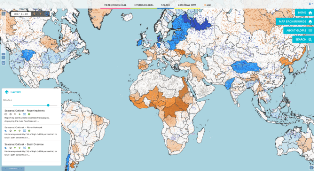
The seasonal outlook is displayed as three new layers in the GloFAS web interface, which is publicly (and freely) available at www.globalfloods.eu. The first of these gives a global overview of the maximum probability of unusually high or low river flow (defined as flow exceeding the 80th or falling below the 20th percentile of the model climatology), during the 4-month forecast horizon, in each of the 306 major world river basins used in GloFAS-Seasonal.

new_web_figure1_basins
The new GloFAS Seasonal Outlook Basin Overview and River Network Layers.

The second layer provides further sub-basin-scale detail, by displaying the global river network (all pixels with an upstream area >1500km2), again coloured according to the maximum probability of unusually high or low river flow during the 4-month forecast horizon. In the third layer, reporting points with global coverage are displayed, where more forecast information is available. At these points, an ensemble hydrograph is provided showing the 4-month forecast of river flow, with thresholds for comparison of the forecast to typical or extreme conditions based on the model climatology. Also displayed is a persistence diagram showing the weekly probability of exceedance for the current and previous three forecasts.

blog_screenshot
The new GloFAS Seasonal Outlook showing the river network and reporting points providing hydrographs and persistence diagrams.

Over the coming months, an evaluation of the system will be completed – for now, users are advised to evaluate the forecasts for their particular application. We welcome any feedback on the forecast visualisations and skill – feel free to contact me at the email address below!

To find out more, you can see the University’s press release here, further information on SEAS5 here, and the user information on the seasonal outlook GloFAS layers here.

*Water@Reading is “a vibrant cross-faculty centre of research excellence at the University of Reading, delivering world class knowledge in water science, policy and societal impacts for the UK and internationally.”

Full list of collaborators: 

Rebecca Emerton1,2, Ervin Zsoter1,2, Louise Arnal1,2, Prof. Hannah Cloke1, Dr. Liz Stephens1, Dr. Florian Pappenberger2, Prof. Christel Prudhomme2, Dr Peter Salamon3, Davide Muraro3, Gabriele Mantovani3

1 University of Reading
2 ECMWF
3 European Commission JRC

Contact: r.e.emerton@pgr.reading.ac.uk

Clear-Air Turbulence and Climate Change

Europe_turbulence_blog
Figure 1: Percentage change of clear-air turbulence over Europe and the North Atlantic

Clear-Air Turbulence (CAT) is a major hazard to the aviation industry. If you have ever been on a plane you have probably heard the pilots warn that clear-air turbulence could occur at any time so always wear your seatbelt. Most people will have experienced it for themselves and wanted to grip their seat. However, severe turbulence capable of causing serious passenger injuries is rare. It is defined as the vertical motion of the aircraft being strong enough to force anyone not seat belted to leave the chair or floor if they are standing. In the United States alone, it costs over 200 million US dollars in compensation for injuries, with people being hospitalised with broken bones and head injuries. Besides passengers suffering serious injuries, the cabin crew are most vulnerable as they spend most of the time on their feet serving customers. This results in an additional cost if they are injured and unable to work.

Clear-air turbulence is defined as high altitude inflight bumpiness away from thunderstorm activity. It can appear out of nowhere at any time and is particularly dangerous because pilots can’t see or detect it using on-board instruments.  Usually the first time a pilot is aware of the turbulence is when they are already flying through it. Because it is a major hazard, we need to know how it might change in the future, so that the industry can prepare if necessary. This could be done by trying to improve forecasts so that pilots can avoid regions likely to contain severe turbulence or making sure the aircraft can withstand more frequent and severe turbulence.

Our new paper published in Geophysical Research Letters named ‘Global Response of Clear-Air Turbulence to Climate Change’ aims at understanding how clear-air turbulence will change in the future around the world and throughout the year. What our study found was that, the busiest flight routes around the world would see the largest increase in turbulence. For example, the North Atlantic, North America, North Pacific and Europe (see Figure 1) will see a significant increase in severe turbulence which could cause more problems in the future. These regions see the largest increase because of the Jet Stream. The Jet Stream is a fast flowing river of air that is found in the mid-latitudes. Clear-air turbulence is predominantly caused by the wind traveling at different speeds around the Jet Stream. Climate change is expected to increase the Jet Stream speed and therefore increase the vertical wind shear, causing more turbulence.

To put these findings in context, severe turbulence in the future will be as frequent as moderate turbulence historically. Anyone who is a frequent flyer will have likely experienced moderate turbulence at some point, but fewer people have experienced severe turbulence. Therefore, this study suggests this will change in the future with most frequent flyers experiencing severe turbulence on some flight routes as well as even more moderate turbulence. Our study also found moderate turbulence will become as frequent in the summer as it has done historically in winter. This is significant because although clear-air turbulence is more likely in winter, it will however now become much more of a year round phenomenon (see Figure 2).

Seasonal_turbulence_blog
Figure 2: Percentage change of clear-air turbulence around the world in all four seasons. No Stipling (stipling) indicates it is (is not) significant at the 90% confidence level.

This increase in clear-air turbulence highlights the importance for improving turbulence forecasting. Current research has shown that using ensemble forecasts (many forecasts of the same event) and also using more turbulence diagnostics than the one we used in this study can improve the forecast skill. By improving the forecasts, we could consistently avoid the areas of severe turbulence or make sure passengers and crew are seat-belted before the turbulence event occurs. Unfortunately, as these improvements are not yet fully operational, you can still reduce your own risk of injury by making sure you wear your seat belt as much as possible so that, if the aircraft does hit unexpected turbulence, you would avoid serious injuries.

Storer, L. N., Williams, P. D., & Joshi, M. M. (2017). Global response of clear-air turbulence to climate change. Geophysical Research Letters, 44, 99769984. https://doi.org/10.1002/2017GL074618

This blog was originaly writen for EGU Blogs