Between the 11th-16th March myself and four other PhDs and post docs attended the Ocean in Weather and Climate (OiWC) course at the Met Office, Exeter. This NERC advanced training course was aimed at PhDs, postdocs and beyond. It provided a great opportunity to spend a week meeting other Oceanography researchers at varying stages of their career, and to expand your understanding of the oceans role in climate beyond the scope of your own work.
The week kicked off with an ice breaker where we had do some ‘Scientific speed dating’, chatting to other participants about: Where are you from? What do you work on? What is your main hobby? What is the biggest question in your field of research? This set the tone for a very interactive week full of interesting discussions between all attendees and speakers alike. Course participants were accommodated at The Globe Inn situated in Topsham, a cute village-sized town full of pastel-coloured houses, cosy pubs, art galleries, and beautiful riverside walks to stretch your legs in the evenings.
The days consisted of four 1.5 hour sessions, split up by caffeine and biscuit breaks to recharge before the next session.
Topics covered in the lecture-style talks included…
Dynamical Theory
Modelling the Ocean
Observations
Ocean-atmosphere coupling
Air-sea fluxes
High Resolution Ocean modelling in coupled forecast systems
The Meridional Overturning Circulation
The Southern Ocean in climate and climatic change
Climate variability on diurnal, seasonal, annual, inter-annual, decadal timescales
Climate extremes
Climate sensitivity, heat uptake and sea level.
A recurring figure of the week…. taken from Helene Hewitt’s talk on high resolution ocean modelling showing ocean surface currents from HadGEM3-based global coupled models at different resolutions (eddy resolving, eddy permitting and eddy parameterised).
All the talks were very interesting and were followed by some stimulating discussion. Each session provided an overview of each topic and an indication of the current research questions in each area at the moment.
In the post lunch session, there were group practical sessions. These explored observational ARGO float data and model output. The practicals, written in iPython notebooks, were designed to let us play with some data, giving us a series of questions to trigger group discussions to deepen understanding of topics covered that morning.
The course also included some ‘softer’ evening talks, giving research career advice in a more informal manner. Most evenings were spent exploring the lovely riverside walks and restaurants/pubs of Topsham. The final evening was spent all together at the Cosy Club in Exeter, rounding off a very interesting and enjoyable week!
Online comic “xkcd” set a trend for explaining complicated things using only the 1000 most common words when they created this schematic of Saturn-V. They have subsequently published more on how microwaves, plate tectonics and your computer work, using the same style.
So we thought we’d jump on the bandwagon in a recent PhD group meeting, and have a go at explaining our research topics using the ten-hundred most common words. You can have a go yourselves, and tweet us with it @SocialMetwork on Twitter. Enjoy!
The Role of the Asian Summer Monsoon in European Summer Climate Variability – Jonathan Beverley
I look at how heavy rain in in-dear in summer makes rain, sun, wind and other things happen in your-up. This happens by big waves high up in the sky moving around the world. We might be able to use this to make a long know-before better and to help people live longer and not lose money.
Contribution of near-infrared bands of greenhouse gases to radiative forcing – Rachael Byrom
I study how the sun’s light warms the sky. This happens when these really tiny things in the air that we can’t see eat the sun’s light which then makes the sky warmer. I use computers to look into how this happens, especially how exactly the really tiny things eat the sun’s light and how this leads to warming. By this I mean, if I add lots of the tiny things to a pretend computer sky, all over the world, then will the sky also warm over all of the world too and by how much will it warm? This might be interesting for people who lead the world so that they can see how much of the really tiny things we should be allowed to put into the sky.
Wind profile effects on gravity wave drag and their impact on the global atmospheric circulation – Holly Turner
I look at waves in the air over high places and how they slow down the wind. When the wind gets faster the higher up you go, it changes how it slows down. I want to use this to make computer wind pictures better.
To be a doctor, I look at a fire-breathing ground thing with smoke and rocks on a hot place surrounded by water. I look at space pictures to understand the relationships between the air that smells and fire-rock bits in the air, and other stuff. It’s a very angry fire-breathing ground thing and might kill the near-by humans
Surface fluxes, temperatures and boundary layer evolutions in the building grey zone in London – Beth Saunders
I work on numbers which come out of the Met Office’s computer world. These numbers are different to what is seen and felt in real life for cities. True numbers, seen in real life, help to say how hot cities are, and how different the hot city is to areas that aren’t cities, with trees and fields, because of the city’s people, cars and houses. Numbers saying how fast the wind goes, and the wind’s direction, change in cities because of all the areas with tall houses. Finding times where the computer world numbers are bad for cities will help to make the Met Office’s computer give numbers more like the true numbers.
Cloud electrification and lightning in the evolution of convective storms – Ben Courtier
To be a doctor, I look at sudden light shocks from angry water air that happens with noise in the sky and how the angry water air changes before the light shock happens. I do this in order to better guess when the sudden light shock happens.
Politics. Science. They are two worlds apart. One is about trying to understand and reveal the true nature of the universe using empirical evidence. The other is more invested in constructing its own reality; cherry-picking evidence which conforms to the desired perception of the universe. Ok, so this is a gross simplification. Politicians have by no means an easy task. They are expected to make huge decisions on limited evidence and understanding. Meanwhile, whilst we all like the romantic idea that the science we do is empirical and non-biased, there are frequent examples (such as the perils of the impact factor or sexism in peer review) to counter this. We do understand, however, that evidence lies at the core of what we do. A good research paper will highlight what evidence has led to a conclusion or outcome, how that evidence was collected, and any uncertainties or limitations of the evidence. This is essential for transparency and reproducibility. What if we could introduce the same tools to politics?
For effective public scrutiny of policies, transparency in how evidence is used is essential. Credit for photo: Jamie Smith, Unsplash
In October 2017 I spent multiple hours reviewing government policy documents to assess just how well they were using evidence. I was contributing to the Sense about Science publication transparency of evidence: spot check. This document is the product of a collaboration in 2015 between Sense about Science, the Institute for Government and the Alliance for Useful Evidence wherein the evidence transparency framework was proposed. This framework aims to encourage government to be transparent in their use of evidence. In November 2016, Sense about Science published the original transparency of evidence report which was a trial use of this framework applied to a random selection of ‘publicly-available policy documents’. After feedback from the departments and participants involved, the framework has been refined to produce the spot check.
The review involved a team of young scientists, including me, each assessing how a subset of around 10 of these policies is using evidence. At this stage the quality of this evidence, or whether the policy has merit based on the presented evidence, was not considered. The priority is to assess the transparency in how evidence is being used to shape policy. We scored each policy in four key areas (with a score out of 3 given for each area):
Diagnosis: The policymakers should outline all they know about a particular issue including its causes, impacts and scale with supporting evidence. Any uncertainties or weaknesses in the evidence base should be highlighted.
Proposal: The policy should outline the chosen intervention with a clear statement of why this approach has been selected as well as any negatives. It should also be made clear why other approaches have not been used, and if the chosen intervention has not been fully decided on how the Government intends to make that decision. Once again the strengths and weaknesses of the evidence base should be acknowledged and discussed.
Implementation: If the method for implementing the proposal has not been made, what evidence will be used to make that decision? If it has, why has this approach been selected over alternatives, and what negatives exist? As previously, supporting evidence should be provided and assessed for its quality.
Testing and Evaluation: Will there be a pilot / trial of the policy and if not why not? How will the impacts and outcomes of the policy be assessed? The testing methods and criteria for success should be made clear, with an accompanying timetable.
For full details of this framework refer to Appendix 1 of the transparency of evidence: spot check publication. Whilst the framework is fairly explicit, it was nevertheless challenging as a reviewer to provide a fair assessment of each policy. The policies ranged in content from cyber-security to packaging waste; some were a few pages long, some closer to 100 pages; some were still at the consultation stage and others were ready to implement. Furthermore, sometimes values and pragmatism are as important in policy making as the available evidence. Policies based on such values can still be scored highly provided it is explicit and justified why these values have taken priority over any available contradictory evidence.
The findings discussed within the report are consistent with what I found when reviewing the policies. In particular, whilst inclusion of supporting evidence has improved since the original assessment, an approach of “info-dumping” seems to have been adopted whereby evidence is provided without being explicit about why it is relevant or it has been used. Similarly often references are cited without it being clear why. Many policies also failed to make the chain of reasoning from diagnosis to testing and evaluation of a policy clear. These complaints should not be unfamiliar to scientists! Finally, very few documents discussed how policies would be tested and evaluated. I am hoping by this point it should be clear why we as scientists can have a positive input. The same skills we use to produce high quality research and papers can be used to produce transparent and testable policies.
We have established why a scheme to engage young researchers in assessing and improving use of evidence in policy making has value, however perhaps you may still be wondering why we should care? Linking back to the theme of this blog, in the next few years we are going to see a raft of policies worldwide designed to combat climate change in response to the Paris Agreement. As the people providing the evidence, climate scientists will have a role in scrutinising these policies and ensuring they will achieve the predicted outcomes. For this to happen, transparency of evidence is essential. Furthermore, we all exist as citizens outside of our research, and as citizens we should want the ability to properly hold government and other policy makers accountable.
This year the Department of Meteorology are participating and organising several events to raise money for the David Grimes Trust, a part of Reading San Francisco Libre Association. The David Grimes Trust was set-up after the passing away of Dr. David Grimes, a Reader in African Meteorology and an integral part of our department. His works include leading the TAMSAT group from the mid-1990s and supporting a new generation of African scientists. More details about David Grimes and the Reading San Francisco Libre can be found at http://www.met.reading.ac.uk/david/ and http://www.sanfranciscolibre.org/.
Events taking place include a departmental bake sale and a Meteorology Gatsby Ball. 20 members of the department are also running the Reading Half Marathon, and you can support them by donating at https://mydonate.bt.com/fundraisers/metdeptreadinghalf2018 .
This week’s blog post comes from Nick Byrne, a recent PhD graduate from the department, who’s written a two-day diary for us on his experiences in Nicaragua visiting San Francisco Libre.
Day 1
05:30 – Days in Nicaragua begin early! In San Francisco Libre (and in ‘el campo’ in general) everyone is up from as early as 04.00. Animals are tended to and tortillas are prepared from scratch, perhaps also along with a dish of ‘gallo pinto’ and some coffee.
School in San Francisco Libre
In the big towns life begins a little later. I’m staying in Esteli, a city in the northern highlands which is over 100km from SFL. My ‘expreso’ bus to Managua leaves at 06.45 and I only have time for a banana before I have to dash out the door.
08:00 – The bus drops me at the side of the highway near San Benito where I need to catch a regular bus to SFL. I get some travel advice from a friendly owner of a nearby ‘pulperia’, who tells me that the bus should arrive in about an hour. Regular buses in Nicaragua (or ‘chicken buses’ to tourists) are often retired American schoolbuses that have been redecorated in colourful ways. Anything and everything can be sold on them, and a couple of fresh Nicaraguan ‘picos’ can be very welcome if you missed breakfast.
11:00 – The bus arrives in SFL! I get off outside the house of a German NGO where 4 young volunteers are spending the year. I meet two of them, Flo and Clara, before being introduced to local resident and president of APREDEN (Association for the Recovery and Development of the Environment in Nicaragua), Jimmy Zamora. I give Jimmy a small gift of art supplies from Reading which he tells me will be very popular with the children of SFL. We chat briefly with the volunteers at the house and then hop on Jimmy’s bike for a ride to the local ‘comedor’ where we get some food and a delicious melon ‘fresco’.
12:00 – Over lunch we talk about some recent projects in SFL such as the plant nursery and beekeeping programs in ‘La Guayabita’, and the education programs in the library and the school. Between working on the various projects and coordinating activities with the German NGO, Jimmy is effectively on duty 24/7. Like many Nicaraguans, participating in his church community and singing in the choir at weekends is his release from the challenges that work brings. We also talk a little about his visit to England and his love of The Beatles, and we even manage a brief discussion on how residents perceive climate change in SFL.
13:00 – After lunch we spend the afternoon visiting various projects and activities in SFL. These include the harbour and canal network to the capital Managua, the semi-developed volcanic bath and spa facility for tourists, and also to the many communities surrounding the lake that were devastated by flooding after hurricane Mitch and from heavy rains in recent years. A recurrent theme is that even in difficult conditions, SFL is not lacking in creative solutions to the various problems that arise. The primary challenge is finding funding to get a project started. I’m told that the average daily wage for an agricultural worker in Nicaragua is around $5 a day, and so even a few dollars can have a huge impact on the daily quality of life.
Perhaps the project which Jimmy and colleagues are most proud of is the work at ‘La Guayabita’. This is a nursery for plants and trees as well as housing the location of the beekeeping project in SFL. There is a close connection between both of these projects as the bees help pollinate the nursery, while a diverse ecological system is crucial for a successful beekeeping program. When the beekeeping program initially started, all that the community had was the technical expertise of a few residents. Over time, and with the help of various fundraising efforts (including from the David Grimes Trust in Reading), the necessary materials were purchased and now the program is actually generating money for the community.
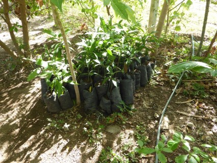
Plants at La Guayabita
The nursery itself has a striking visual impact as deforestation has been a problem in SFL over recent decades. Plants from the nursery are being used to redevelop recently bought land and this major project is currently in the early stages of development. Jimmy’s colleagues describe it best by calling ‘La Guayabita’ the lungs of SFL.
17:00 – Saturday evening is a chance to unwind a little. A karaoke competition has been organised in the central park and many children and families are present to enjoy the atmosphere. Jimmy is hosting the event and there is a wide range of genres. Songs range from recent hits such as ‘Chambea’ and ‘Casate Conmigo’ to crowdpleasers like ‘Me Gusta Tu Vieja’ (which I’m told is a Mexican joke about ‘your mum’!). Jimmy closes the event with a ranchera called ‘La Ley De La Vida’ before the prizes are presented. Everyone goes home around 21.00 after a very enjoyable evening.
Day 2
5:30 – I wake with the roosters and have breakfast with the German volunteers. We talk about their experience, from the initial shock of their first few weeks, to their determination to make the most of their year-long stay, to them now being an integral part of community life. They are well-known amongst the children of SFL, who like to chat and play whenever they pass the house. After breakfast I meet Jimmy again, and we go to visit the school and library education projects.
9:00 – The selection of books and educational materials in the library is impressive, and both the school and the library have been colourfully decorated with many art projects from the school children along with flowers and trees from the surrounding gardens. The library also contains materials for a weather station funded by the David Grimes Trust, along with English teaching materials donated by Caversham resident Russell Maddicks during a recent visit. Jimmy tells me that the project that they are currently working on in the library is to raise money for a sound system so that regular dance classes and audio lessons can be held. This is likely to cost a couple of hundred dollars and so it may be sometime before the project is finally completed.
Donated English Materials
The Library
11:00 – Suddenly it is 11.00 and we realise that it is time for me to leave. I say some quick goodbyes and then hop on Jimmy’s bike for the hour drive down the ’41’ from where I will catch my bus back to Esteli. I’m very grateful to Jimmy for taking the time to drive me personally, and this kindness is a typical example of what I have experienced from everyone in SFL during my short visit. It’s been a fantastic experience to meet a community I’ve read so much about since I came to Reading; after getting to know someone as committed to community work as Jimmy, it is much easier to understand how fundraising efforts in Reading can be translated into real community impacts thousands of miles away in SFL. I tell Jimmy that I hope to be able to visit again on my way home to Ireland in a couple of weeks, and he informs me that I should be just in time to sample some freshly harvested honey!
Morning School.
Morning School.
Thank you to Jimmy Zamora and volunteers for providing photos.
Modes of variability are climatological features that have global effects on regional climate and weather. They are identified through spatial structures and the timeseries associated with them (so-called EOF/PC analysis, which finds the largest variability of a given atmospheric field). Examples of modes of variability include El Niño Southern Oscillation, Madden-Julian Oscillation, North Atlantic Oscillation, Annular modes, etc. The latter are named after the “annulus” (a region bounded by two concentric circles) as they occur in the Earth’s midlatitudes (a band of atmosphere bounded by the polar and tropical regions, Fig. 1), and are the most important modes of midlatitude variability, generally representing 20-30% of the variability in a field.
Figure 1: Southern Hemisphere midlatitudes (red concentric circles) as annulus, region where annular modes have the largest impacts. Source.
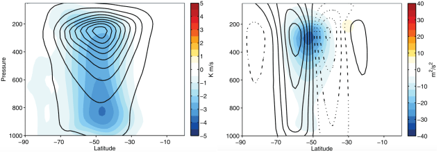
We know two types of annular modes: baroclinic (based on eddy kinetic energy, a proxy for eddy activity and an indicator of storm-track intensity) and barotropic (based on zonal mean zonal wind, representing the north-south shifts of the jet stream) (Fig. 2). The latter are usually referred to as Southern (SAM or Antarctic Oscillation) or Northern (NAM or Arctic Oscillation) Annular Mode (depending on the hemisphere), have generally quasi-barotropic (uniform) vertical structure, and impact the temperature variations, sea-ice distribution, and storm paths in both hemispheres with timescales of about 10 days. The former are referred to as BAM (baroclinic annular mode) and exhibit strong vertical structure associated with strong vertical wind shear (baroclinicity), and their impacts are yet to be determined (e.g. Thompson and Barnes 2014, Marshall et al. 2017). These two modes of variability are linked to the key processes of the midlatitude tropospheric dynamics that are involved in the growth (baroclinic processes) and decay (barotropic processes) of midlatitude storms. The growth stage of the midlatitude storms is conventionally associated with increase in eddy kinetic energy (EKE) and the decay stage with decrease in EKE.
Figure 2: Barotropic annular mode (right), based on zonal wind (contours), associated with eddy momentum flux (shading); Baroclinic annular mode (left), based on eddy kinetic energy (contours), associated with eddy heat flux (shading). Source: Thompson and Woodworth (2014).
However, recent observational studies (e.g. Thompson and Woodworth 2014) have suggested decoupling of baroclinic and barotropic components of atmospheric variability in the Southern Hemisphere (i.e. no correlation between the BAM and SAM) and a simpler formulation of the EKE budget that only depends on eddy heat fluxes and BAM (Thompson et al. 2017). Using cross-spectrum analysis, we empirically test the validity of the suggested relationship between EKE and heat flux at different timescales (Boljka et al. 2018). Two different relationships are identified in Fig. 3: 1) a regime where EKE and eddy heat flux relationship holds well (periods longer than 10 days; intermediate timescale); and 2) a regime where this relationship breaks down (periods shorter than 10 days; synoptic timescale). For the relationship to hold (by construction), the imaginary part of the cross-spectrum must follow the angular frequency line and the real part must be constant. This is only true at the intermediate timescales. Hence, the suggested decoupling of baroclinic and barotropic components found in Thompson and Woodworth (2014) only works at intermediate timescales. This is consistent with our theoretical model (Boljka and Shepherd 2018), which predicts decoupling under synoptic temporal and spatial averaging. At synoptic timescales, processes such as barotropic momentum fluxes (closely related to the latitudinal shifts in the jet stream) contribute to the variability in EKE. This is consistent with the dynamics of storms that occur on timescales shorter than 10 days (e.g. Simmons and Hoskins 1978). This is further discussed in Boljka et al. (2018).
Figure 3: Imaginary (black solid line) and Real (grey solid line) parts of cross-spectrum between EKE and eddy heat flux. Black dashed line shows the angular frequency (if the tested relationship holds, the imaginary part of cross-spectrum follows this line), the red line distinguishes between the two frequency regimes discussed in text. Source: Boljka et al. (2018).
References
Boljka, L., and T. G. Shepherd, 2018: A multiscale asymptotic theory of extratropical wave, mean-flow interaction. J. Atmos. Sci., in press.
Boljka, L., T. G. Shepherd, and M. Blackburn, 2018: On the coupling between barotropic and baroclinic modes of extratropical atmospheric variability. J. Atmos. Sci., in review.
Marshall, G. J., D. W. J. Thompson, and M. R. van den Broeke, 2017: The signature of Southern Hemisphere atmospheric circulation patterns in Antarctic precipitation. Geophys. Res. Lett., 44, 11,580–11,589.
Simmons, A. J., and B. J. Hoskins, 1978: The life cycles of some nonlinear baroclinic waves. J. Atmos. Sci., 35, 414–432.
Thompson, D. W. J., and E. A. Barnes, 2014: Periodic variability in the large-scale Southern Hemisphere atmospheric circulation. Science, 343, 641–645.
Thompson, D. W. J., B. R. Crow, and E. A. Barnes, 2017: Intraseasonal periodicity in the Southern Hemisphere circulation on regional spatial scales. J. Atmos. Sci., 74, 865–877.
Thompson, D. W. J., and J. D. Woodworth, 2014: Barotropic and baroclinic annular variability in the Southern Hemisphere. J. Atmos. Sci., 71, 1480–1493.
Earth’s radiation belts are a hazardous environment for the satellites underpinning our everyday life. The behaviour of these high-energy particles, trapped by Earth’s magnetic field, is partly determined by the existence of plasma waves. These waves provide the mechanisms by which energy and momentum are transferred and particle populations physically moved around, and it’s some of these waves that I study in my PhD.
However, I’ve noticed that whenever I talk about my work, I rarely talk about where this plasma comes from. In schools it’s often taught that space is a vacuum, and while it is closer to a vacuum than anything we can make on Earth, there are enough particles to make it a dangerous environment. A significant amount of particles do escape from Earth’s ionosphere into the magnetosphere but in this post I’ll focus on material entering from the solar wind. This constant outflow of hot particles from the Sun is a plasma, a fluid where enough of the particles are ionised that the behaviour of the fluid is then dominated by electric and magnetic fields. Since the charged particles in a plasma interact with each other, with external electric and magnetic fields, and also generate more fields by moving and interacting, this makes for some weird and wonderful behaviour.
Figure 1: The area of space dominated by Earth’s magnetic field (the magnetosphere) is shaped by the constant flow of the solar wind (a plasma predominantly composed of protons, electrons and alpha particles). Plasma inside the magnetosphere collects in specific areas; the radiation belts are particularly of interest as particles there pose a danger to satellites. Credit: NASA/Goddard/Aaron Kaas
When explaining my work to family or friends, I often describe Earth’s magnetic field as a shield to the solar wind. Because the solar wind is well ionised, it is highly conductive, and this means that approximately, the magnetic field is “frozen in” to the plasma. If the magnetic field changes, the plasma follows this change. Similarly, if the plasma flows somewhere, the magnetic field is dragged along with it. (This is known as Alfvén’s frozen in theorem – the amount of plasma in a volume parallel to the magnetic field line remains constant). And this is why the magnetosphere acts as shield to all this energy streaming out of the Sun – while the magnetic field embedded in the solar wind is topologically distinct from the magnetic field of the Earth, there is no plasma transfer across magnetic field lines, and it streams past our planet (although this dynamic pressure still compresses the plasma of the magnetosphere, giving it that typical asymmetric shape in Figure 1).
Of course, the question still remains of how the solar wind plasma enters the Earth’s magnetic field if such a shielding effect exists. You may have noticed in Figure 1 that there are gaps in the shield that the Earth’s dipole magnetic field presents to the solar wind; these are called the cusps, and at these locations the magnetic field connects to the solar wind. Here, plasma can travel along magnetic field lines and impact us on Earth.
But there’s also a more interesting phenomenon occurring – on a small enough scale (i.e. the very thin boundaries between two magnetic domains) the assumptions behind the frozen-in theorem break down, and then we start to see one of the processes that make the magnetosphere such a complex, fascinating and dynamic system to study. Say we have two regions of plasma with opposing orientation of the magnetic field. Then in a middle area these opposing field lines will suddenly snap to a new configuration, allowing them to peel off and away from this tightly packed central region. Figure 2 illustrates this process – you can see that after pushing red and blue field lines together, they suddenly jump to a new configuration. As well as changing the topology of the magnetic field, the plasma at the centre is energised and accelerated, shooting off along the magnetic field lines. Of course even this is a simplification; the whole process is somewhat more messy in reality and I for one don’t really understand how the field can suddenly “snap” to a new configuration.
Figure 2: Magnetic reconnection. Two magnetic domains of opposing orientation can undergo a process where the field line configuration suddenly resets. Instead of two distinct magnetic domains, some field lines are suddenly connected to both, and shoot outwards and away, as does the energised plasma.
In the Earth’s magnetosphere there are two main regions where this process is important (Figure 3). Firstly, at the nose of the magnetosphere. The dynamic pressure of the solar wind is compressing the solar wind plasma against the magnetospheric plasma, and when the interplanetary magnetic field is orientated downwards (i.e. opposite to the Earth’s dipole – about half the time) this reconnection can happen. At this point field lines that were solely connected to the Earth or in the solar wind are now connected to both, and plasma can flow along them.
Figure 3: There are two main areas where reconnection happens in Earth’s magnetosphere. Opposing field lines can reconnect, allowing a continual dynamic cycle (the Dungey cycle) of field lines around the magnetosphere. Plasma can travel along these magnetic field lines freely. Credits: NASA/MMS (image) and NASA/Goddard Space Flight Center- Conceptual Image Lab (video)
Then, as the solar wind continues to rush outwards from the Sun, it drags these field lines along with it, past the Earth and into the tail of the magnetosphere. Eventually the build-up of these field lines reaches a critical point in the tail, and boom! Reconnection happens once more. You get a blast of energised plasma shooting along the magnetic field (this gives us the aurora) and the topology has rearranged to separate the magnetic fields of the Earth and solar wind; once more, they are distinct. These dipole field lines move around to the front of the Earth again, to begin this dramatic cycle once more.
Working out when and how these kind of processes take place is still an active area of research, let alone understanding exactly what we expect this new plasma to do when it arrives. If it doesn’t give us a beautiful show of the aurora, will it bounce around the radiation belts, trapped in the stronger magnetic fields near the Earth? Or if it’s not so high energy as that, will it settle in the cooler plasmasphere, to rotate with the Earth and be shaped as the magnetic field is distorted by solar wind variations? Right now I look out my window at a peaceful sunny day and find it incredible that such complicated and dynamic processes are continually happening so (relatively) nearby. It certainly makes space physics an interesting area of research.
Reproducing the result of a scientific experiment is necessary to establish trust, and reproducibility has long been a key part of the scientific method. Traditionally, an experiment could be repeated by following the method documented by the original scientists: setting up apparatus, taking measurements, and so on. If the method was sufficiently well documented then it was, perhaps, likely that the original results could be reproduced. These ‘wet lab’ experiments continue today, but many experiments are now performed entirely on computers. Such computational experiments involve no physical apparatus, but merely the processing of input data files through some scientific software before writing more data files for later analysis and plotting.
Repeating computational experiments is particularly difficult because, before any results can be obtained, there are many pieces of software apparatus that must be assembled: we must install an operating system, choose the correct version of our programming language and all the necessary scientific libraries, and we must use input parameters that are identical to those used in the original experiment. Assembling any of these pieces incorrectly might lead to subtly incorrect results, obviously incorrect results, or a failure to obtain any results at all. All this places a burden on the original scientists to document every piece of software, its version number and input parameters, and places a burden on the scientist wishing to reproduce the results.
There are a variety of tools that help to relieve this burden by automating the process of conducting computational experiments. Singularity is one such tool, having been purpose-built for automating computational experiments. A scientist creates a single configuration file that provides all the information Singularity needs to assemble the pieces of software apparatus and perform the experiment. This way, instead of writing a ‘method’ section that is only human-readable, the scientist has written a configuration file that is both human-readable and machine-readable. Using this configuration, Singularity will create an image file with all the correct versions of scientific software pre-installed. The scientist can verify their work by reproducing their experiment themselves, and they can run the same experiment just by copying the image file between their personal laptop, office workstation, or their institution’s HPC cluster. And they can send their Singularity configuration file and image files to other scientists, or they can obtain a DOI by uploading the files to Zenodo, making their computational experiments citeable in the same way as their journal publications.
I’ve used Singularity to run my own atmospheric simulations using the OpenFOAM computational fluid dynamics software. While my results have yet to be reproduced by others, I regularly use Singularity to reproduce my own results on my laptop, university desktop and AWS cloud compute servers, giving me confidence that my software and my results are robust. Whenever I’ve been stuck, the friendly Singularity developers have been quick to help out on twitter. But overall, I’ve found Singularity to be easy to use, and anyone that is familiar with git commands should feel right at home using it. Give it a try!
Joseph Taylor, NERC SCEARNIO DTP student. Zoological Society of London.
Email: J.Taylor5@pgr.reading.ac.uk
Projecting the impacts of climate change on biodiversity is important for informing
Male Mauritius kestrel (Falco punctatus) in the Bambous Mountains, eastern Mauritius. Photo by Joe Taylor.
mitigation and adaptation strategies. There are many studies that project climate change impacts on biodiversity; however, changes in the occurrence of extreme weather events are often omitted, usually because of insufficient understanding of their ecological impacts. Yet, changes in the frequency and intensity of extreme weather events may pose a greater threat to ecosystems than changes in average weather regimes (Jentsch and Beierkuhnlein 2008). Island species are expected to be particularly vulnerable to climate change pressures, owing to their inherently limited distribution, population size and genetic diversity, and because of existing impacts from human activities, including habitat destruction and the introduction of non-native species (e.g. Fordham and Brook 2010).
Mauritius is an icon both of species extinction and the successful recovery of threatened species. However, the achievements made through dedicated conservation work and the investment of substantial resources may be jeopardised by future climate change. Conservation programmes in Mauritius have involved the collection of extensive data on individual animals, creating detailed longitudinal datasets. These provide the opportunity to conduct in-depth analyses into the factors that drive population trends.
My study focuses on the demographic impacts of weather conditions, including extreme events, on three globally threatened bird species that are endemic to Mauritius. I extended previous research into weather impacts on the Mauritius kestrel (Falco punctatus), and applied similar methods to the echo parakeet (Psittacula eques) and Mauritius fody (Foudia rubra). The kestrel and parakeet were both nearly lost entirely in the 1970s and 1980s respectively, having suffered severe population bottlenecks, but all three species have benefitted from successful recovery programmes. I analysed breeding success using generalised linear mixed models and analysed survival probability using capture-mark-recapture models. Established weather indices were adapted for use in this study, including indices to quantify extreme rainfall, droughts and tropical cyclone activity. Trends in weather indices at key conservation sites were also analysed.
The results for the Mauritius kestrel add to a body of evidence showing that precipitation is an important limiting factor in its demography and population dynamics. The focal population in the Bambous Mountains of eastern Mauritius occupies an area in which rainfall is increasing. This trend could have implications for the population, as my analyses provide evidence that heavy rainfall during the brood phase of nests reduces breeding success, and that prolonged spells of rain in the cyclone season negatively impact the survival of juveniles. This probably occurs through reductions in hunting efficiency, time available for hunting and prey availability, so that kestrels are unable to capture enough prey to sustain themselves and feed their young (Nicoll et al. 2003, Senapathi et al. 2011). Exposure to heavy and prolonged rainfall could also be a direct cause of mortality through hypothermia, especially for chicks if nests are flooded (Senapathi et al. 2011). Future management of this species may need to incorporate strategies to mitigate the impacts of increasing rainfall.
References:
Fordham, D. A. and Brook, B. W. (2010) Why tropical island endemics are acutely susceptible to global change. Biodiversity and Conservation 19(2): 329‒342.
Jentsch, A. and Beierkuhnlein, C. (2008) Research frontiers in climate change: Effects of extreme meteorological events on ecosystems. Comptes Rendus Geoscience 340: 621‒628.
Nicoll, M. A. C., Jones, C. G. and Norris, K. (2003) Declining survival rates in a reintroduced population of the Mauritius kestrel: evidence for non-linear density dependence and environmental stochasticity. Journal of Animal Ecology 72: 917‒926.
Senapathi, D., Nicoll, M. A. C., Teplitsky, C., Jones, C. G. and Norris, K. (2011) Climate change and the risks associated with delayed breeding in a tropical wild bird population. Proceedings of the Royal Society B 278: 3184‒3190.