1st Met Office Training and Research Summer School

Email: carlo.cafaro@pgr.reading.ac.uk

From the last week of June until the 1st September I took part in the Met Office Training and Research (MOTR), as part of the Mathematics of Planet Earth CDT.

Inspired by the highly popular and successful Geophysical Fluid Dynamics Summer School at the Woods Hole Oceanographic Insitution in the USA, it is a 10 week-programme, hosted by Met Office in Exeter. The PhD students have the opportunity to handle an applied research topic outside the area of their PhD, diversify their portfolio and experience the working and social life at the Met Office.

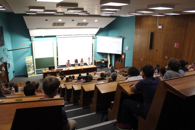
In the first two weeks we participated in a summer school. In particular in the first week there was a lecture course on ”Regional Climate Variability and Change”. In the morning the lectures were given by David Karoly from University of Melbourne on “patterns of climate change”, starting from the basic concepts of the climate systems and then expanding to the climate change attribution. In the afternoon we had specialist lectures by Met Office and University of Exeter scientists about El Nino, modelling paleoclimates and attribution of extreme weather events. 

IMG-20170630-WA0001
David Karoly giving one of his lecture on attribution of regional climate change patterns.

In addition, in the afternoon we had to do lab work working in pairs, using Climate Explorer, choosing a specific continent of the world and investigating past climate and future climate projections for that area. My colleague and I selected South America and we gave a presentation about that.

During the second week we participated in the workshop ”Future opportunities to inform UK regional projections”, with a lecture given by Ed Hawkins, amongst  others, talking about sources of uncertainty.

From the third week onward each student started a research project in different Met Office research groups. A different colleague and I worked within the Atmospheric Processes and Parametrization group (APP), supervised by Gabriel Rooney. My project was on numerical simulations and theoretical aspects of colliding density currents. Other colleagues were placed within the Climate Science, Dynamics groups and Informatics Lab, a partner of Met Office.

A typical day for us at Met Office started at 9am, meeting almost every day with Gabriel at 9.45 am, coffee break at 10.30 for half an hour or so (where I also met Annelize, previously in Reading), 1 hour lunch break and then “working” again until 5.30 pm or so.

WP_20170710_19_20_06_Pro
Not quite our typical day at Met Office (found on a desk at Met Office)

Also, once a week we had the meeting with the smaller convection group, where everyone was asked to give an update of their own work. We also attended journal club sessions on Fridays and a brainstorming meeting on 21st July. It was nice to take part in these events, even being only summer interns. During the project phase we had also weekly advanced seminars by Glenn Shutts and Mike Cullen, mainly about large-scale dynamics and hierarchies of operational models used in NWP.

WP_20170721_10_34_41_Pro
Glenn Shutts giving a lecture on Rossby waves breaking.

Personally, it was a wonderful experience for several reasons. The Met Office is a very pleasant place to work, with very friendly and flexible people. Since I think my project was quite academic I did not find many differences with working at university itself. Nevertheless, interacting with new people in a new environment has provided me with new inspirations and insights. I had the chance to talk with several scientists and also a chief Meteorologist, since I was curious about the activities carried out in the Operational room and how much communication there is with the research side. There were some social and sports events organised by MOSSA (Met Office Social and Sports Association) which I really enjoyed (picnic and sports day), getting the chance to meet and to talk with people of other research divisions.

Finally, to top it off, I visited Exeter a lot and the area around, mainly during the weekends and the 5 days of holidays agreed at the beginning, even going to Cornwall for 2 days. 

In the end I would like to thank all of the organisers, my supervisor and all the people I talked with for giving me and my colleagues this very valuable opportunity which I will keep always in mind for my future career.

Thunderstorms and showers: an insight into UK operational radar rainfall estimation.

If there’s one thing you can count on in Britain it’s that at any given time someone, somewhere, is talking about rain.  Either it’s raining, or we want it to rain, or it absolutely mustn’t be raining today.  It’s just one of those things we love to complain about – and we do!

My work isn’t in forecasting rain, but observing it. It’s a little known fact that the rainfall map you see on the front page of the Met Office website doesn’t just come straight out of one giant weather radar, neatly packaged.  There’s a lot of work that has to happen before we can turn the “reflectivities” from many different radar echoes into a sensible estimate of how heavily it’s raining on your street.

The Met Office owns and manages a network of 15 weather radars across the UK, and receives data from three more, in Ireland and the Channel Islands.  We’ve now almost completed a major upgrade of the network, replacing key components of the old radars – some of which had been running operationally for over 30 years! – with new technology.  The dual polarisation and Doppler information we obtain from the upgraded radars improves our ability to distinguish between “rain” and “non-rain” echoes, and to measure how fast the rain is moving, feeding improvements in short range “nowcasts” and flood forecasting models. It can also help us estimate the quantity of rainfall and other types of precipitation in real time.

For my PhD, I’m looking at how to improve Met Office estimates of surface rain rates from radar measurements at long range.  When a radar measures weather, it does so with a beam of energy that spreads out with distance.  20 km from the radar, the echo received represents a volume of space around 600 m by 400 m by 400 m.  At 50 km, the volume is 600 m by 1 km squared.  By 100 km, the beam has spread out to be 2 km wide.  This effect is called “beam broadening”, and limits the spatial detail with which we can measure rainfall.

The other effect of range is the increasing height of the radar beam above the ground.  This means the radar isn’t always measuring liquid rain drops, but may be measuring frozen ice crystals or snow, high up in colder parts of the atmosphere, which will melt before they reach the surface.  Snow, melting snow and rain all have different reflectivities, so we have to correct for this “vertical profile” to calculate how much rain is falling at ground level.

The Met Office corrects for the vertical reflectivity profile (VPR) using an iterative scheme (Kitchen et al. 1994, Kitchen 1997).  We know roughly the VPR shape, and the amount of beam broadening at a given range, so we can scale this shape to the actual radar reflectivity measurement.  This allows us to correct for the impacts of melting snow, which causes a huge enhancement of the radar measurement and would – if uncorrected – lead to extreme overestimates of rainfall.  In the early days of weather radar, this caused rings of very high rain rates to appear in the image: an effect called “bright banding”.  VPR correction also compensates for the underestimation of rain rates at very long distances from the radar.

201410131416_stratiform_rhi
Vertical slice “range height indicator” scan of rain from October 2014.  There is a “bright band” at 2 km height due to melting snowflakes in the reflectivity and linear depolarisation ratio (LDR).

In my work, I’m using measurements from the upgraded dual polarisation radar network to choose between different VPR shapes in making this correction.  Specifically, I’m investigating the depolarising properties of different melting drops, to identify the rare situations where we don’t need to correct for “bright banding”.  The linear depolarisation ratio (LDR), which I’m using to identify the large melting snowflakes that cause radar bright bands, has to be measured using different scans from the ones used to collect reflectivities for rainfall rates, and the Met Office is one of very few meteorological services capable of measuring LDR operationally.  Using LDR in this way can improve rainfall estimates significantly in cases where there is no bright band (Smyth and Illingworth, 1998; Sandford et al., in press).

201507032220_convective_rhi
Vertical slice “range height indicator” scan of a convective shower from July 2015.  There is no bright band in reflectivity, and very little melting layer enhancement in LDR.

As a logical extension to this work, I’m also looking into new VPR shapes for “non-bright band” rain, using vertical slice “range height indicator” scans from our research radar at Wardon Hill.  Correction for bright band is well established in the radar literature, as this is the most common type of rain at high latitudes (where the freezing level is low enough to affect radar measurements), but other types of VPR (e.g. Fabry and Zawadzki, 1995) are rarely discussed.  With the improvements in classification achieved by the new LDR algorithm, a suitable VPR shape is needed to correct for underestimation far from the radar in cases without bright band.  I’ve recently developed a test profile shape for non-bright band VPRs, and demonstrated improvements to rain rates in localised convective case studies. The method is currently being trialled for use in the Met Office’s operational radar processing software.

In the future it’s hoped that the work I’m doing will further improve the accuracy of Met Office rainfall estimates, particularly in thunderstorms and convective showers. And when the weather is doing things like this, that’s good to know!

References

Fabry, F. and I. Zawadzki, 1995: Long-term radar observations of the melting layer of precipitation and their interpretation. Journal of the Atmospheric Sciences, 52, 838-851.

Kitchen, M., 1997: Towards improved radar estimates of surface precipitation rate at long range. Quarterly Journal of the Royal Meteorological Society, 123, 145-163.

Kitchen, M., R. Brown. and A. Davies, 1994: Real-time correction of weather radar data for the effects of bright band, range and orographic growth in widespread precipitation. Quarterly Journal of the Royal Meteorological Society, 120, 1231-1254.

Sandford, C., A. Illingworth, and R. Thompson, in press: The potential use of the linear depolarisation ratio to distinguish between convective and stratiform rainfall to improve radar rain rate estimates. Journal of Applied Meteorology and Climatology.

Smyth, T. and A. Illingworth, 1998: Radar estimates of rainfall rates at the ground in bright band and non-bright band events. Quarterly Journal of the Royal Meteorological Society, 124, 2417-2434.

Surviving the Viva

Email: d.l.a.flack@reading.ac.uk

Recently in the department we have had a fair number of students submitting their PhD theses and awaiting or completing their viva.

For many students at the start of the PhD the viva seems a long way off and can often be thought of as a terrifying experience. So why then do many PhD students come out of their viva saying that they enjoyed it? and is it really as XKCD portray it?

MY RESULTS ARE A SIGNIFICANT IMPROVEMENT ON THE STATE OF THE AAAAAAAAAAAART
Thesis defense according to XKCD

With the help of some former PhD students (Hannah Bloomfield, Sammie Buzzard, Hannah Gough and Leo Saffin) we’ve come up with a summary of our own experiences and some advice for people just about to go in.

But before I get into that I’ll briefly explain a little bit about the viva. The viva is (alongside writing the thesis) the examination for the PhD. Its essentially an oral exam where you sit and talk about your thesis and the area surrounding your field. The viva can last anywhere between 90 minutes and 5 hours, depending on how much you have to talk about (and how much you or your examiners talk). The result from the viva is as follows: Fail; Major Corrections requiring another viva; Pass: Major corrections; Pass: Minor corrections (the most common) and Pass: No corrections (very rare), and at the end of the day it’s the pass or fail that matters.

So what can you expect from a viva? Well, as with each PhD each viva is different (hence why this post is a collaborative effort). Even people’s nerves are different, some go in feeling confident, whilst others are still fairly nervous about it (which of course is very understandable). I certainly was in the nervous camp, but I would have been disappointed if I wasn’t because I always feel I perform better if I am nervous beforehand. Indeed, many of us who are initially nervous become relaxed as soon as we get into the swing of things and the questions start flowing. Furthermore, many examiners (not all) will know and understand that you will be nervous so will immediately put you at ease by saying something along the lines of “I really enjoyed reading your thesis and you don’t need to be worried about the result.” This last statement is probably key for anyone going into the viva – by the time it gets to the viva your examiners have already decided the result, the viva is mainly to check that you did the work.

Looking at the recent experiences of the PhD students I have broadly classified the viva into three types, Presentation,Traditional” and Thesis covering described below.

Presentation (Hannah Gough):

Hannah was asked to produce a presentation for her viva. She did find this useful as it was a good way to settle into the viva and bring across the aims and key conclusions of her thesis, at the same time highlight what she felt was the most important figures in her thesis. After the presentation, the examiners asked questions on her entire thesis. These ranged from points of clarification, to the wider implications of her work.

Traditional” (Hannah Bloomfield, Sammie Buzzard and Leo Saffin):

The more “traditional” viva asks you to summarise your thesis for the first 3-5 minutes and then goes through the thesis asking about wider implications and where your work fits in, basic theory, parts of the thesis they are unsure about and implications of your work (amongst other things).

Thesis covering (myself):

Essentially, all we did was go through my thesis cover-to-cover discussing bits specifically related to my project (some minor wider implications/knowledge) and comments that they had on my work.

So why do people enjoy the viva then? Well, there is a fairly simple answer to this question. You’ve been doing work for between three and four years and now you get to discuss it in detail and the examiner can see that you know what you are talking about and will often ask some interesting and thought provoking questions that you either haven’t considered or didn’t necessarily view as important.

Other things that are worth mentioning about the viva, before going on to our collective advice, is that most of the time (unless you spend a while talking about basics of your area) the viva doesn’t feel it is taking as long as it actually is (2 hours feels like 15 minutes – I’m not just saying that, it really does!) – it’s essentially the old saying “time flies when you are having fun”.

So, that’s a brief overview of the viva and our experiences, so how do you actually survive it? Our collective advice would be as follows:

  1. You are the expert in your thesis – so don’t panic – your examiners don’t know as much about what you did as you do.
  2. The examiners are not there to trick you, they are just checking that you did your work – they’ve already made the pass/fail decision.
  3. Don’t be afraid to ask for breaks from time to time (your examiners may want a break too).
  4. Don’t look at the clock (if there is one in the room). All you will then do is think about how long you have been in the viva.
  5. Bring food (biscuits, etc) and enough to share with your examiners.
  6. Prepare a simple 3-5 minute overview of your thesis and know it well – generally you will be asked to summarise your thesis.
  7. It can be useful to read a couple of your external examiners papers – just to find out a little bit about them at the very least.
  8. Don’t be afraid to ask questions to be explained in more detail so you know exactly what they want.
  9. Eat something before you go in no matter how bad you feel.
  10. Try and get a good night’s sleep beforehand.
  11. Don’t be afraid to say how you would do things differently, after having had time to look back at it.
  12. You are the expert in your thesis – so don’t panic – your examiners don’t know as much about what you did as you do.

With that all I can say if you are facing a viva soon is good luck.

A special thanks to all the former PhD students that helped provide information for this blog: Hannah Gough, Hannah Bloomfield, Samantha Buzzard and Leo Saffin.

Should we be ‘Leaf’-ing out vegetation when parameterising the aerodynamic properties of urban areas?

Email: C.W.Kent@pgr.reading.ac.uk

When modelling urban areas, vegetation is often ignored in attempt to simplify an already complex problem. However, vegetation is present in all urban environments and it is not going anywhere… For reasons ranging from sustainability to improvements in human well-being, green spaces are increasingly becoming part of urban planning agendas. Incorporating vegetation is therefore a key part of modelling urban climates. Vegetation provides numerous (dis)services in the urban environment, each of which requires individual attention (Salmond et al. 2016). However, one of my research interests is how vegetation influences the aerodynamic properties of urban areas.

Two aerodynamic parameters can be used to represent the aerodynamic properties of a surface: the zero-plane displacement (zd) and aerodynamic roughness length (z0). The zero-plane displacement is the vertical displacement of the wind-speed profile due to the presence of surface roughness elements. The aerodynamic roughness length is a length scale which describes the magnitude of surface roughness. Together they help define the shape and form of the wind-speed profile which is expected above a surface (Fig. 1).

blogpostpic

Figure 1: Representation of the wind-speed profile above a group of roughness elements. The black dots represent an idealised logarithmic wind-speed profile which is determined using the zero-plane displacement (zd) and aerodynamic roughness length (z0) (lines) of the surface.

For an urban site, zd and z0 may be determined using three categories of methods: reference-based, morphometric and anemometric. Reference-based methods require a comparison of the site to previously published pictures or look up tables (e.g. Grimmond and Oke 1999); morphometric methods describe zd and z0 as a function of roughness-element geometry; and, anemometric methods use in-situ observations. The aerodynamic parameters of a site may vary considerably depending upon which of these methods are used, but efforts are being made to understand which parameters are most appropriate to use for accurate wind-speed estimations (Kent et al. 2017a).

Within the morphometric category (i.e. using roughness-element geometry) sophisticated methods have been developed for buildings or vegetation only. However, until recently no method existed to describe the effects of both buildings and vegetation in combination. A recent development overcomes this, whereby the heights of all roughness elements are considered alongside a porosity correction for vegetation (Kent et al. 2017b). Specifically, the porosity correction is applied to the space occupied and drag exerted by vegetation.

The development is assessed across several areas typical of a European city, ranging from a densely-built city centre to an urban park. The results demonstrate that where buildings are the dominant roughness elements (i.e. taller and occupying more space), vegetation does not obviously influence the calculated geometry of the surface, nor the aerodynamic parameters and the estimated wind speed. However, as vegetation begins to occupy a greater amount of space and becomes as tall as (or larger) than buildings, the influence of vegetation is obvious. Expectedly, the implications are greatest in an urban park, where overlooking vegetation means that wind speeds may be slowed by up to a factor of three.

Up to now, experiments such as those in the wind tunnel focus upon buildings or trees in isolation. Certainly, future experiments which consider both buildings and vegetation will be valuable to continue to understand the interaction within and between these roughness elements, in addition to assessing the parameterisation.

References

Grimmond CSB, Oke TR (1999) Aerodynamic properties of urban areas derived from analysis of surface form. J Appl Meteorol and Clim 38:1262-1292.

Kent CW, Grimmond CSB, Barlow J, Gatey D, Kotthaus S, Lindberg F, Halios CH (2017a) Evaluation of Urban Local-Scale Aerodynamic Parameters: Implications for the Vertical Profile of Wind Speed and for Source Areas. Boundary-Layer Meteorology 164: 183-213.

Kent CW, Grimmond CSB, Gatey D (2017b) Aerodynamic roughness parameters in cities: Inclusion of vegetation. Journal of Wind Engineering and Industrial Aerodynamics 169: 168-176.

Salmond JA, Tadaki M, Vardoulakis S, Arbuthnott K, Coutts A, Demuzere M, Dirks KN, Heaviside C, Lim S, Macintyre H (2016) Health and climate related ecosystem services provided by street trees in the urban environment. Environ Health 15:95.

5th WGNE workshop on systematic errors in weather and climate models

The 5th Working Group on Numerical Experimentation (WGNE) workshop on systematic errors in weather and climate models was held in Montréal, Canada from 19 to 23 June 2017. The principal goal of the workshop is to increase understanding of the nature and cause of errors in models used for weather and climate prediction, including intra-seasonal to inter-annual scales.

IMG_20170618_204314
Centre Mont-Royal, venue for the workshop

The workshop is held every four years. The 5th WGNE workshop focused on processes that models currently fail to represent accurately, based around six themes: atmosphere-land-ocean-cryosphere interactions, clouds and precipitation, resolution issues, teleconnections, metrics and diagnostics, and model errors in ensembles. For each of the themes, the workshop started off with talks from invited keynote speakers, followed by contributed oral presentations, a conclusion session and a poster session.

My PhD project studies mean-state precipitation biases over the Maritime Continent in CMIP5 atmosphere-only experiments, which aligns well with the “model errors in ensembles” workshop theme. I received a lot of constructive feedback and suggestions during the discussions in the poster session.

IMG_20170622_132821379
Lunch with experts. Photo courtesy of Ariane Frassoni
IMG_20170621_200054892
Pub night. Photo courtesy of Ariane Frassoni

A mixture of scientific and social activities were organized in this workshop dedicated to Early Career Scientists (ECS). We had the opportunity to be a session rapporteur and participate in a best poster competition. Then we were given the chance to get to know more established scientists during the more social ‘lunch-with-experts’ and ‘pub night’ activities. The lunch-with-experts was truly entertaining – with conversations about PhD life and challenges, future career path advice, variations between countries in PhD education systems and much more! ECS were also given the opportunity to become co-reviewer of a poster competition session where we work in pairs with an expert scientist to review posters in a session we are not competing in. By becoming the co-reviewer, we get to experience the review process and get in contact with expert scientists.

IMG_20170623_121858669
Session rapporteur presentation. Photo courtesy of Ariane Frassoni

On the last day, the session rapporteur presented a summary on the main issues discussed in each session, followed by a panel discussion and an overall conclusion to the workshop. I am very happy that my poster on ‘Maritime Continent seasonal climate biases in AMIP experiments of the CMIP5 multimodel ensemble’ was given the Best Poster Award, alongside with Falko Judt for his poster on ‘Effect of model error on the predictability of hurricane intensity’ and Danahé Paquin-Ricard for her poster on ‘The role and impact of a deep convective parameterization on Km-scale atmospheric forecasts’ during the closing session.

IMG_20170623_133016499
ECS group photo. Photo courtesy of Ariane Frassoni

Lastly, I also got to do some sightseeing while I was in Montréal after the workshop. From the amazing Notre-Dame Basilica, great views of the city from Mont Royal and the underground city to escape the weather, Montréal has so much to offer!


I am thankful to the World Meteorological Organization (WMO) for providing me the travel funding to attend the workshop and present my poster. Also many thanks go to Ariane Frassoni for organising the pub nights and facilitating the ECS activities, as well as for providing the photos for this post.

Two Weeks in Paris Learning about Fluid Dynamics and Sampling French Pastries

Email: r.frew@pgr.reading.ac.uk

The Fluid Dynamics of Sustainability and the Environment (FDSE) residential summer school runs every summer for two weeks, alternating between Cambridge University and Ecole polytechnique, which run the summer school in partnership. I attended this years hosted by Ecole polytechnique, situated to the South of Paris. 40 PhD students attended from institutes around the world, all working on a range of topics who want to learn more about environmental fluid dynamics.

logo-wake-green

The lectures covered topics on fundamentals of fluid dynamics, flow instabilities, environmental fluid dynamics, cryosphere, atmosphere, physical oceanography and renewable energy. The lectures went at a very fast pace (approximately triple speed!), aiming to familiarise us with as many concepts as possible in the two weeks, resulting in everyone taking home a large overflowing folder full of lecture notes to refer back to in the future.

We were kept very busy throughout the two weeks. Each day started with breakfast (coffee and croissants) between 7.30-8.20 am, followed by two back to back lectures 8.30-10.30 am. There was then half an hour for everyone to fuel their brain with coffee and (warm!) mini pastries before another hour lecture before lunch break. Lunch was roughly 12-1.30 pm, although typically there were so many interesting questions after each lecture that we ran progressively later relative to the schedule meaning that I think we only actually started lunch on time on the first day. There were also a number of guest speakers speaking on topics such as public engagement, climate policy, meteorology on mars and air quality.

After lunch we had the final lecture of the day, followed by a short break before numerical sessions and lab experiments, which ran until roughly 6 pm. These sessions gave us the chance to really learn about a particular topic in more detail and to have a more hands on experience with some of the material being lectured. My labs were on tidal energy where we explored the energy output and efficiency of tidal turbines, and Art and Science, which encouraged us to engage with Science in new and more playful ways and also to challenge us to look at it differently.

However the day didn’t end after the labs, the evenings were also jam packed! The first evening was a poster session, giving us all the opportunity to learn more about what all of the other students work on and to mingle. Other evenings consisted of learning to row sessions, visits to the observatory, movie nights and discussions about the ‘science’ in The Day After Tomorrow movie and barbeques enjoying the warm light evenings (definitely missing those now I’m back in Reading).

During the weekend sandwiched in the middle of the two weeks, we were all transferred to a hostel in the centre of Paris, setting us all up perfectly for some weekend sightseeing in Paris. On the Friday evening there was a boat party reception on the Siene, supplying us all with lots of wine, many difference French cheeses to sample and a lively dance floor.

The school ended on Friday July 14th, Bastille Day. After a morning presenting a few slides on the labs we had completed in groups to share what we had learnt, we travelled into the centre of Paris ready for an evening enjoying the spectacular Bastille Day fireworks around the Eiffel tower, ending the summer school with a bang.

Personally the main take away from the summer school was not to learn the entirety of the lecture content, but to become familiar with a wide range of topics gain more hands on experience of laboratory experiments and to have a (rather large) folder full of lecture notes to refer back to whenever I stumble across a particular concept again in the future. And of course, it was great having the opportunity to meet lots of other PhD students from around the world working on related topics and to be able to discuss, engage and get to know each other over the two weeks. I would like to thank all of the organisers and lecturers of the summer school for a really interesting and enjoyable two weeks!


Future of Cumulus Parametrization conference, Delft, July 10-14, 2017

Email: m.muetzelfeldt@pgr.reading.ac.uk

For a small city, Delft punches above its weight. It is famous for many things, including its celebrated Delftware (Figure 1). It was also the birthplace of one of the Dutch masters, Johannes Vermeer, who coincidentally painted some fine cityscapes with cumulus clouds in them (Figure 2). There is a university of technology with some impressive architecture (Figure 3). It holds the dubious honour of being the location of the first assassination using a pistol (or so we were told by our tour guide), when William of Orange was shot in 1584. To this list, it can now add hosting a one-week conference on the future of cumulus parametrization, and hopefully bringing about more of these conferences in the future.

Delftware_display

Figure 1: Delftware.

Vermeer-view-of-delft

Figure 2: Delft with canopy of cumulus clouds. By Johannes Vermeer, 1661.

Delft_AULA

Figure 3: AULA conference centre at Delft University of Technology – where we were based for the duration of the conference.

So what is a cumulus parametrization scheme? The key idea is as follows. Numerical weather and climate models work by splitting the atmosphere into a grid, with a corresponding grid length representing the length of each of the grid cells. By solving equations that govern how the wind, pressure and heating interact, models can then be used to predict what the weather will be like days in advance in the case of weather modelling. Or a model can predict how the climate will react to any forcings over longer timescales. However, any phenomena that are substantially smaller than this grid scale will not be “seen” by the models. For example, a large cumulonimbus cloud may have a horizontal extent of around 2km, whereas individual grid cells could be 50km in the case of a climate model. A cumulonimbus cloud will therefore not be explicitly modelled, but it will still have an effect on the grid cell in which it is located – in terms of how much heating and moistening it produces at different levels. To capture this effect, the clouds are parametrized, that is, the vertical profile of the heating and moistening due to the clouds are calculated based on the conditions in the grid cell, and this then affects the grid-scale values of these variables. A similar idea applies for shallow cumulus clouds, such as the cumulus humilis in Vermeer’s painting (Figure 2), or present-day Delft (Figure 3).

These cumulus parametrization schemes are a large source of uncertainty in current weather and climate models. The conference was aimed at bringing together the community of modellers working on these schemes, and working out which might be the best directions to go in to improve these schemes, and consequently weather and climate models.

Each day was a mixture of listening to presentations, looking at posters and breakout discussion groups in the afternoon, as well as plenty of time for coffee and meeting new people. The presentations covered a lot of ground: from presenting work on state-of-the-art parametrization schemes, to looking at how the schemes perform in operational models, to focusing on one small aspect of a scheme and modelling how that behaves in a high resolution model (50m resolution) that can explicitly model individual clouds. The posters were a great chance to see the in-depth work that had been done, and to talk to and exchange ideas with other scientists.

Certain ideas for improving the parametrization schemes resurfaced repeatedly. The need for scale-awareness, where the response of the parametrization scheme takes into account the model resolution, was discussed. One idea for doing this was the use of stochastic schemes to represent the uncertainty of the number of clouds in a given grid cell. The concept of memory also cropped up – where the scheme remembers if it had been active at a given grid cell in a previous point in time. This also ties into the idea of transitions between cloud regimes, e.g. when a stratocumulus layer splits up into individual cumulus clouds. Many other, sometimes esoteric, concepts were discussed, such as the role of cold pools, how much tuning of climate models is desirable and acceptable, how we should test our schemes, and what the process of developing the schemes should look like.

In the breakout groups, everyone was encouraged to contribute, which made for an inclusive atmosphere in which all points of view were taken on board. Some of the key points of agreement from these were that it was a good idea to have these conferences, and we should do it more often! Hopefully, in two years’ time, another PhD student will write a post on how the next meeting has gone. We also agreed that it would be beneficial to be able to share data from our different high resolution runs, as well as to be able to compare code for the different schemes.

The conference provided a picture of what the current thinking on cumulus parametrization is, as well as which directions people think are promising for the future. It also provided a means for the community to come together and discuss ideas for how to improve these schemes, and how to collaborate more closely with future projects such as ParaCon and HD(CP)2.

Experiences of the NERC Atmospheric Pollution and Human Health Project.

Email: k.m.milczewska@pgr.reading.ac.uk

One of the most exciting opportunities of my PhD experience to date has been a research trip to Beijing in June, as part of the NERC Atmospheric Pollution and Human Health (APHH) project. This is a worldwide research collaboration with a focus on the way air pollution in developing megacities affects human health, and the meeting in Beijing served as the 3rd project update.

Industrialisation of these cities in the last couple of decades has caused air pollution to rise rapidly and regularly exceed levels deemed safe by the World Health Organisation (WHO).  China sees over 1,000,000 deaths annually due to particulate matter (PM), with 76 deaths per 100,000 capita. In comparison, the UK has just over 16,000 total deaths and 26 per capita. But not only do these two countries have very different climates and emissions; they are also at very different stages of industrial development. So in order to better understand the many various sources of pollution in developing megacities – be they from local transport, coal burning or advected from further afield – there is an increased need for developing robust air quality (AQ) monitoring measures.

The APHH programme exists as a means to try and overcome these challenges. My part in the meeting was to expand the cohort of NCAS / NERC students researching AQ in both the UK and China, attending a series of presentations in a conference-style environment and visiting two sites with AQ monitoring instruments. One is situated in the Beijing city centre while the other in the rural village of Pinggu, just NW of Beijing. Over 100 local villagers take part in a health study by carrying a personal monitor with them over a period of two weeks. Their general health is monitored at the Pinggu site, alongside analysis of the data collected about their personal exposure to pollutants each day, i.e. heatmaps of different pollutant species are created according to GPS tracking. Having all the instruments being explained to us by local researchers was incredibly useful, because since I work with models, I haven’t had a great deal of first hand exposure to pollutant data collection. It was beneficial to get an appreciation of the kind of work this involves!

IMG_8121

In between all our academic activities we also had the chance to take some cultural breaks – Beijing has a lot to offer! For example, our afternoon visit to the Pinggu rural site followed the morning climb up the Chinese Great Wall. Although the landscape was somewhat obscured by the pollution haze, this proved to be a positive thing as we didn’t have to suffer in the direct beam of the sun!


I would like to greatly thank NERC, NCAS and University of Leeds for the funding and organisation of this trip. It has been an incredible experience, and I am looking forward to observing the progess of these projects, hopefully using what I have learnt in some of my own work.

For more information, please visit the APHH student blog in which all the participants documented their experiences: https://www.ncas.ac.uk/en/introduction-to-atmospheric-science-home/18-news/2742-ncas-phd-students-visit-four-year-air-quality-fieldwork-project-in-beijing