By Maia Arama (m.arama@pgr.reading.ac.uk), Molly Macrae(molly.macrae@pgr.reading.ac.uk) and Giacomo Giuliani (g.giuliani@pgr.reading.ac.uk)
A big part of doing a PhD at Reading is the opportunity to complete training courses that expand our skillsets and knowledge. Below, we summarise and review our experiences of different courses offered by the National Centre for Atmospheric Science (NCAS) that we completed at the beginning of our PhDs.
Introduction to Scientific Computing (ISC), Maia Arama
In November 2025, I completed the ISC course run by NCAS. The course consisted of three modules designed to provide students with essential skills and tools for data analysis. Module 1 introduced Linux commands, Module 2 covered an introduction to Python programming, and Module 3 focused on data analysis tools in Python (e.g. numpy, x-array, cf-python). Modules 1 and 2 were aimed at beginners, while Module 3 was aimed at those with some prior experience. After completing a short quiz, I was able to skip Module 2 and complete only Modules 1 and 3. Module 1 was delivered online while Modules 2 and 3 were taught at NCAS headquarters in Leeds.
The most valuable things I learned from Module 1 was how to combine commands using pipes and filters, as well as writing loops and shell scripts. I now regularly use these skills to process data for my PhD project! I did find that more time was spent on easier sections, while more challenging sections felt rushed at times. However, all material was made available to us on Software Carpentry enabling us to practice with the resources after the module. In Module 3, I found it particularly useful to learn how to use cf-python and cf-plot. We also completed a challenge using weather API data where we created NetCDF files, combined our data and produced a plot. The module also introduced version control with Git and the use of remote GitHub repositories. All teaching was done using Jupyter Notebooks on Jasmin.
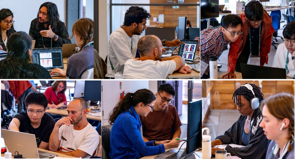
Overall, I had a fantastic experience attending the course in Leeds. The staff were readily available to answer questions and help with debugging code. It was also great to meet other friendly and motivated PhD students, which created an inspiring working environment. Those with more experience in Python may find some of the material quite basic. However, if you have limited coding experience or want to increase your confidence coding in Python, I would highly recommend this course!
Links to the relevant NCAS ISC GitHub pages can be found here:
Module 1: https://ncasuk.github.io/ncas-isc-shell/06a-environment-variables/index.html
Module 3: https://github.com/ncasuk/ncas-isc/
Introduction to the UK Chemistry-Aerosol (UKCA) Model, Molly Macrae
UKCA is a community atmospheric chemistry–aerosol model used to study how atmospheric chemistry, aerosols, and climate interact within the Met Office Unified Model, supporting research on climate forcing, air quality, and ozone processes. The ‘Introduction to UK Chemistry Aerosol (UKCA) Model’ course aims to provide experience of running the model through a set of practical, self-paced tutorials. The course was free to attend and took place in-person in Leeds with accommodation, travel and food included.
Over the 3 days, you are provided with a login to Monsoon3 and work through online tutorials at your own pace with expert UKCA users on hand to answer any questions or help with technical issues. These tutorials covered how to use the main parts of the UKCA model, setting up and running experiments, and how to adapt the model to specific purposes. There were also pre-recorded walkthrough videos provided, which were incredibly useful if anything from the instructions was unclear. Additionally, the logins were made available for a couple of weeks beyond the course, and a Slack channel was set up for any queries that arose after the course.
Despite most of the training being individual, I really appreciated that the course was held in-person. It was a great opportunity to meet other people using UKCA and to get guidance and feedback from the experts about how I plan to use UKCA in my project.
Overall, I found the course very useful, and I still go back to the provided resources now as I run the model. As expected for a course introducing the running of a climate model, there is a lot of information to take in, and after a few months, the elements of the course that have stayed with me are the parts I am actually using the model for now. Furthermore, the resources provided are clear and available for returning to at a later date. The self-paced format also allows you to tailor the course by spending longer on tutorials most relevant to your research. I would strongly recommend this course to anyone considering using UKCA in their work.
Course webpage with tutorials: UKCA Chemistry and Aerosol Tutorials at UMvn13.9 – UKCA
Introduction to the Unified Model, Giacomo Giuliani
The ‘Introduction to the Unified Model (UM)’ course is a 3-day course organised by NCAS at its headquarters in Leeds. It consists of two complementary parts: a series of lectures on the UM components and their applications, and tutorial sessions focused on working with suites and model outputs.
The UM is the atmospheric model for numerical weather prediction and climate projections. It can be run using different configurations, also called suites. The “how to use it” part mainly focuses on becoming familiar with the (un)intuitive, and sometimes quixotic, architecture of the workflow, as well as how to run simulations. Much of the tutorials involved working on the terminal interface of Archer2 and the UM graphic user interface, in other words, a good refresher for Shell and Bash scripting.
At the end of the course, I proudly scrolled my notebook page of “Commands, Tips and Common Errors when running the UM” noticing how long – and hopefully comprehensive – it was. I think the main takeaway of the course was: to be able to troubleshoot any issues, to create your own model configurations, and to understand the overall process behind a simulation within the UM framework.
The practical part for the UM course can be found on GitHub. Thus, in principle, one could just “learn from home”. However, the lectures are not the only aspect that makes this course extremely valuable. I rapidly assessed in thirty days and several hours between yawns and desperation the amount of time it would take me to complete this course on my own. It was really valuable and helpful to be able to talk to people who develop and use this model every day. On the other hand, this course may be too high-level for a person only interested in using the UM for numerical simulations. It provides a general overview of the architecture of the UM workflow, but it lacks the use of a testbed simulation to simulate a common research situation.
Overall, I would definitely recommend the course to anyone frequently working with the UM, as soon as they have a solid base in Linux.
Here is the link to the GitHub page: https://ncas-cms.github.io/um-training/index.html