Preparing for the assimilation of future ocean-current measurements

By Laura Risley

Ocean data assimilation (DA) is vital. Firstly, it is essential to improving forecasts of ocean variables. Not only that, the interaction between the ocean and atmosphere is key to numerical weather prediction (NWP) as coupled ocean-atmosphere DA schemes are used operationally.  

At present, observations of the ocean currents are not assimilated operationally. This is all set to change, as satellites are being proposed to measure these ocean currents directly. Unfortunately, the operational DA systems are not yet equipped to handle these observations due to some of the assumptions made about the velocities. In my work, we propose the use of alternative velocity variables to prepare for these future ocean current measurements. These will reduce the number of assumptions made about the velocities and is expected to improve the NWP forecasts.

What is DA? 

DA combines observations and a numerical model to give a best estimate of the state of our system – which we call our analysis. This will lead to a better forecast. To quote my lunchtime seminar ‘Everything is better with DA!’

Our model state usually comes from a prior estimate which we refer to as the background. A key component of data assimilation is that the errors present in both sets of data are taken into consideration. These uncertainties are represented by covariance matrices. 

I am particularly interested in variational data assimilation, which formulates the DA problem into a least squares problem. Within variational data assimilation the analysis is performed with a set of variables that differ from the original model variables, called the control variables. After the analysis is found in this new control space, there is a transformation back to the model space. What is the purpose of this transformation? The control variables are chosen such that they can be assumed approximately uncorrelated, reducing the complexity of the data assimilation problem.

Velocity variables in the ocean 

My work is focused on the treatment of the velocities in NEMOVAR. This is the data assimilation software used by the NEMO ocean model, used operationally at the Met Office and ECMWF. In NEMOVAR the velocities are transformed to their unbalanced components, and these are then used as control variables. The unbalanced components of the velocities are highly correlated, therefore contradicting the assumption made about control variables. This would result in suboptimal assimilation of future surface current measurements – therefore we seek alternative velocity control variables. 

The alternative velocity control variables we propose for NEMOVAR are unbalanced streamfunction and velocity potential. This would involve transforming the current control variables, the unbalanced velocities, to these alternative variables using Helmholtz Theorem. This splits a velocity field into its nondivergent (streamfunction) and irrotational (velocity potential) parts. These parts have been suggested by Daley (1993) as more suitable control variables than the velocities themselves. 

Numerical Implications of alternative variables 

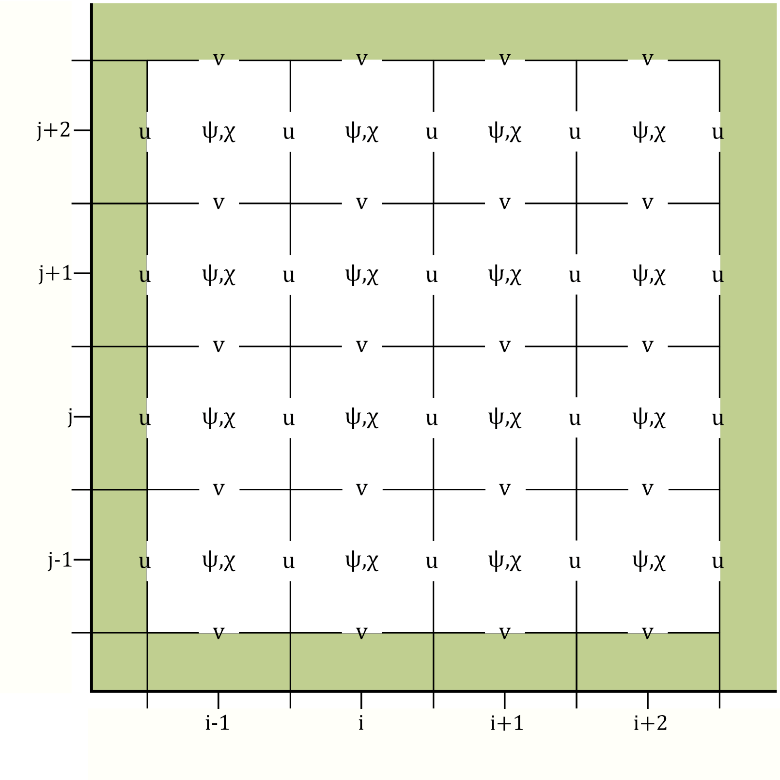
We have performed the transformation to these proposed control variables using the shallow water equations (SWEs) on a 𝛽-plane. To do so we discretised the variables on the Arakawa-C grid. The traditional placement of streamfunction on this grid causes issues with the boundary conditions. Therefore, Li et al. (2006) proposed placing streamfunction in the centre of the grid, as shown in Figure 1. This circumvents the need to impose explicit boundary conditions on streamfunction. However, using this grid configuration leads to numerical issues when transforming from the unbalanced velocities to unbalanced streamfunction and velocity potential. We have analysed these theoretically and here we show some numerical results.

Figure 1: The left figure shows the traditional Arakawa-C configuration (Lynch (1989), Watterson (2001)) whereby streamfunction is in the corner of each grid cell. The right figure shows the Arakawa-C configuration proposed by Li et al. (2006) where streamfunction is in the centre of the grid cell. The green shaded region represents land. 

Issue 1: The checkerboard effect 

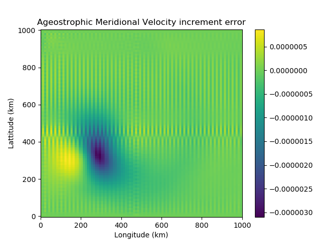
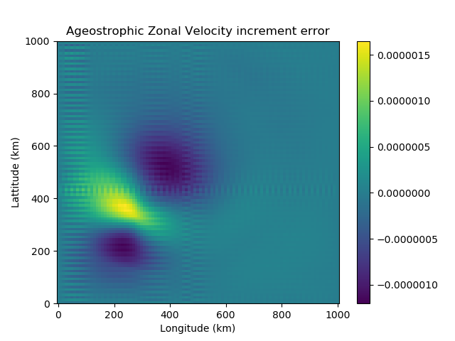
The transformation from the unbalanced velocities to unbalanced streamfunction and velocity potential involves averaging derivatives, due to the location of streamfunction in the grid cell. This process causes a checkerboard effect – whereby we have numerical noise entering the variable fields due to a loss of information. This is clear to see numerically using the SWEs. We use the shallow water model to generate a velocity field. This is transformed to its unbalanced components and then to unbalanced streamfunction and velocity potential. Using Helmholtz Theorem, the unbalanced velocities are reconstructed. Figure 2 shows the checkboard effect clearly in the velocity error.

Figure 2: The difference between the original ageostrophic velocity increments, calculated using the SWEs, and the reconstructed ageostrophic velocity increments. These are reconstructed using Helmholtz Theorem, from the ageostrophic streamfunction and velocity potential increments. On the left we have the zonal velocity increment error and on the right the meridional velocity increment error. 

Issue 2: Challenges in satisfying the Helmholtz Theorem 

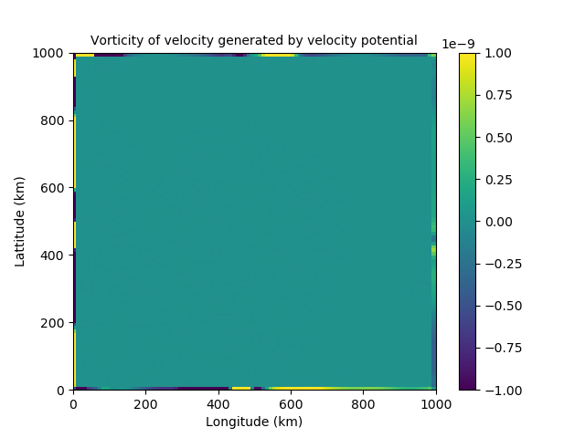
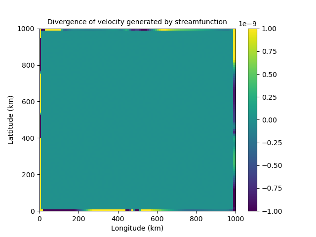
Helmholtz theorem splits the velocity into its nondivergent and irrotational components. We discovered that although streamfunction should be nondivergent and velocity potential should be irrotational, this is not the case at the boundaries, as can be seen in figure 3. This implies the proposed control variables are able to influence each other on the boundary. This would lead to them being strongly coupled and therefore correlated near the boundaries. This directly conflicts the assumption made that our control variables are uncorrelated. 

Figure 3: Issues with Helmholtz Theorem near the boundaries. The left shows the divergence of the velocity field generated by streamfunction. The right shows the vorticity of the velocity field generated by velocity potential. 

Overall, in my work we propose the use of alternative velocity control variables in NEMOVAR, namely unbalanced streamfunction and velocity potential. The use of these variables however leads to several numerical issues that we have identified and discussed. A paper on this work is in preparation, where we discuss some of the potential solutions. Our next work will further this investigation to a more complex domain and assess our proposed control variables in assimilation experiments. 

References: 

Daley, R. (1993) Atmospheric data analysis. No. 2. Cambridge university press. 

Li, Z., Chao, Y. and McWilliams, J. C. (2006) Computation of the streamfunction and velocity potential for limited and irregular domains. Monthly weather review, 134, 3384–3394. 

Lynch, P. (1989) Partitioning the wind in a limited domain. Monthly weather review, 117, 1492–1500. 

Watterson, I. (2001) Decomposition of global ocean currents using a simple iterative method. Journal of Atmospheric and Oceanic Technology, 18, 691–703

Nature vs Nurture in Convective-Scale Ensemble Spread

By Adam Gainford

Quantifying the uncertainty of upcoming weather is now a common procedure thanks to the widespread use of ensemble forecasting. Unlike deterministic forecasts, which show only a single realisation of the upcoming weather, ensemble forecasts predict a range of possible scenarios given the current knowledge of the atmospheric state. This approach allows forecasters to estimate the likelihood of upcoming weather events by simply looking at the frequency of event occurrence within all ensemble members. Additionally, by sampling a greater range of events, this approach highlights plausible worst-case scenarios, which is of particular interest for forecasts of extreme weather. Understanding the realistic range of outcomes is crucial for forecasters to provide informed guidance, and helps us avoid the kind of costly and embarrassing mistakes that are commonly associated with the forecast of “The Great Storm of 1987”*.

To have trust that our ensembles are providing an appropriate range of outputs, we need some method of verifying ensemble spread. We do this by calculating the spread-skill relationship, which essentially just compares the difference between member values to the skill of the ensemble as a whole. If the spread-skill relationship is appropriate, spread and skill scores should be comparable when averaged over many forecasts. If the ensemble shows a tendency to produce larger spread scores than skill scores, there is too much spread and not enough confidence in the ensemble given its accuracy: i.e., the ensemble is overspread. Conversely, if spread scores are smaller than skill scores, the ensemble is too confident and is underspread. 

Figure 1: Postage stamp plots showing three-hourly precipitation accumulation valid for 2023-07-08 09Z at leadtime T+15 h. There is reasonable spread within both the frontal rain band effecting areas of SW England and Wales, and the convective features ahead of this front.

My PhD work has focussed on understanding the spread-skill relationship in convective-scale ensembles. Unlike medium range ensembles that are used to estimate the uncertainty of synoptic-scale weather at daily-to-weekly leadtimes, convective-scale ensembles quantify the uncertainty of smaller-scale weather at hourly-to-daily leadtimes. To do this, convective-scale ensembles must be run at higher resolutions than medium-range ensembles, with grid spacings smaller than 4 km. These higher resolutions allows the ensemble to explicitly represent convective storms, which has been repeatedly shown to produce more accurate forecasts compared coarser-resolution forecasts that must instead rely on convective parametrizations. However, running models at such high resolutions is too computationally expensive to be done over the entire Earth, so they are typically nested inside a lower-resolution “parent” ensemble which provides initial and boundary conditions. Despite this, researchers often report that convective-scale ensembles are underspread, and the range of outputs is too narrow given the ensemble skill. This is corroborated by operational forecasters, who report that the ensemble members often stay too close to the unperturbed control member. 

To provide the necessary context for understanding the underspread problem, many studies have examined the different sources and behaviours of spread within convective-scale ensembles. In general, spread can be produced through three different mechanisms: firstly, through differences in each member’s initial conditions; secondly, through differences in the lateral boundary conditions provided to each member; and thirdly, through the different internal processes used to evolve the state. This last source is really the combination of many different model-specific factors (e.g., stochastic physics schemes, random parameter schemes etc.), but for our purposes this represents the ways in which the convective-scale ensemble produces its own spread. This contrasts with the other two sources of spread, which are directly linked to the spread of the parent ensemble.  

The evolution of each of these three spread sources is shown in Fig. 2. At the start of a forecast, the ensemble spread is entirely dictated by differences in the initial conditions provided to each ensemble member. As we integrate forward in time, though, this initial information is removed from the domain by the prevailing winds and replaced by information arriving through the boundaries. At the same time, internal model processes start spinning up additional detail within each ensemble member. For a UK-sized domain, it takes roughly 12 hours for the initial information to have fully left the domain, though this is of course highly dependent on the strength of the prevailing winds. After this time, spread in the ensemble is partitioned between internal processes and boundary condition differences.  

Figure 2: Attribution of spread within a convective-scale ensemble by leadtime. 

While the exact partitioning in this schematic shouldn’t be taken too literally, it does highlight the important role that the parent ensemble plays in determining spread in the child ensemble. Most studies which try to improve spread target the child ensemble itself, but this schematic shows that these improvements may have quite a limited impact. After all, if the spread of information arriving from the parent ensemble is not sufficient, this may mask or even overwhelm any improvements introduced to the child ensemble.  

However, there are situations where we might expect internal processes to show a more dominant spread contribution. Forecasts of convective storms, for instance, typically show larger spread than forecasts of other types of weather, and are driven more by local processes than larger-scale, external factors.

This is where our “nature” and “nurture” analogy becomes relevant. Given the similarities of this relationship to the common parent-child theory in behavioural psychology, we thought it would be a fun and useful gimmick to also use this terminology here. So, in the “nature” scenario, each child member shows large similarity to the corresponding parent member, which is due to the dominating influence of genetics (initial and boundary conditions). Conversely, in the “nurture” scenario, spread in the child ensemble is produced more by its response to the environment (internal processes), and as such, we see larger differences between each parent-child pair.  

While the nature and nurture attribution is well understood for most variables, few studies have examined the parent-child relationship for precipitation patterns, which are an important output for guidance production and require the use of neighbourhood-based metrics for robust evaluation. Given that this is already quite a long post, I won’t go into too much detail of our results looking at nature vs nurture for precipitation patterns. Instead, I will give a quick summary of what we found: 

  • Nurture provides a larger than average influence on the spread in two situations: during short leadtimes**, and when forecasting convective events driven by continental plume setups. 
  • In the nurture scenarios, spread is consistently larger in the child ensemble than the parent ensemble. 
  • In contrast to the nurture scenarios, nature provides larger than average spread at medium-to-long leadtimes and under mobile regimes, which is consistent with the boundary arguments mentioned previously. 
  • Spread is very similar between the child and parent ensembles in the nurture scenarios.  

If you would like to read more about this work, we will be submitting a draft to QJRMS very soon.  

To conclude, if we want to improve the spread of precipitation patterns in convective-scale ensembles, we should direct more attention to the role of the driving ensemble. It is clear that the exact nesting configuration used has a strong impact on the quality of the spread. This factor is especially important to consider given recent experiments with hectometric-scale ensembles which are themselves nested within convective-scale ensembles. With multiple layers of nesting, the coupling between each ensemble layer is likely to be complex. Our study provides the foundation for investigating these complex interactions in more detail. 

* This storm was actually well forecast by the Met Office. The infamous Michael Fish weather update in which he said there was no hurricane on the way was referring to a different system which indeed did not impact the UK. Nevertheless, this remains a good example of the importance of accurately predicting (and communicating) extreme weather events.  

** While this appears to be inconsistent with Fig. 2, the ensemble we used does not solely take initial conditions from the driving ensemble. Instead, the ensemble uses a separate, high-resolution data assimilation scheme to the parent ensemble. Each ensemble is produced in a way which makes the influence of the data assimilation more influential to the spread than the initial condition perturbations. 

The importance of anticyclonic synoptic eddies for atmospheric block persistence and forecasts

Charlie Suitters – c.c.suitters@pgr.reading.ac.uk

The Beast from the East, the record-breaking winter warmth of February 2020, the Canadian heat dome of 2022…what do these three events have in common? Well, many things I’m sure, but most relevantly for this blog post is that they all coincided with the same phenomenon – atmospheric blocking.

So what exactly is a block? An atmospheric block is a persistent, large-scale, quasi-stationary high-pressure system sometimes found in the mid-latitudes. The prolonged subsidence associated with the high pressure suppresses cloud formation, therefore blocks are often associated with clear, sunny skies, calm winds, and temperature extremes. Their impacts can be diverse, including both extreme heat and extreme cold, drought, poor air quality, and increased energy demand (Kautz et al., 2022). 

Despite the range of hazards that blocking can bring, we still do not fully understand the dynamics that cause a block to start, maintain itself, and decay (Woollings et al., 2018). In reality, many different mechanisms are at play, but the importance of each process can vary between location, season, and individual block events (Miller and Wang, 2022). One process that is known to be important is the interaction between blocks and smaller synoptic-scale transient eddies (Shutts, 1983; Yamazaki and Itoh, 2013). By studying a 43-year climatology of atmospheric blocks and their anticyclonic eddies (both defined by regions of anomalously high 500 hPa geopotential height), I have found that on average, longer blocks absorb more synoptic anticyclones, which “tops up their anticyclonicness” and allows them to persist longer (Fig. 1).

Figure 1: average number of anticyclonic eddies per block for the Euro-Atlantic (left) and North Pacific (right). Block persistence is defined as the quartiles (Q1, Q2, Q3) of all blocks in winter (blue) and summer (red). From Suitters et al. (2023).

It’s great that we now know this relationship, however it would be beneficial to know if these interactions are forecasted well. If they are not, it might explain our shortcomings in predicting the longevity of a block event (Ferranti et al., 2015).  I explore this with a case study from March 2021 using ensemble forecasts from MOGREPS-G. Fortunately, this block in March 2021 was not associated with any severe weather, but it was still not forecasted well. In Figure 2, I show normalised errors in the strength, size, and location of the block, at the time of block onset, for each ensemble member from a range of different initialisation times. In these plots, a negative (positive) value means that the block was forecast to be too weak (strong) or too small (large), and the larger the error in the location, the further away the forecast block was from reality. In general, the onset of this block was forecast to be to be too weak and too small, though there was considerable spread within the ensemble (Fig. 2). Certainty in the forecast was only achieved at relatively small lead times.

Figure 2: Normalised errors in the intensity (left), area (centre), and location of the block’s centre of mass (right), at a validity time of 2021-03-14 12 UTC (the time of onset). Each ensemble member’s error from a particular initialisation time is shown by the grey dots, and the ensemble mean is shown in black. When Z, A, or L are zero, the forecast has a “perfect” replication for this metric of the block (when compared to ERA5 reanalysis).

Now for the interesting bit – what causes the uncertainty in forecasting of the onset this European blocking event? To examine this, I grouped forecast members from an initialisation time of 8 March 2021 according to their ability to replicate the real block: the entire MOGREPS-G mean, members that either have no block or a very small block (Group G), members that perform best (Group H), and members that predict area well, but have the block in the wrong location (Group I). Then, I take the mean geopotential height anomalies (
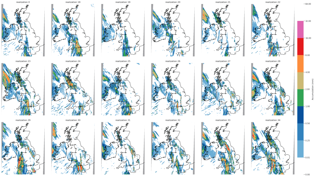
) at each time step in each group, and compare these fields between groups to see if I can find a source of forecast error.

This is shown as an animation in Fig. 3. The animation starts at the time of block onset, and goes back in time to selected validity times, as shown at the top of the figure. The domain of the plot also changes in each frame, gradually moving westwards across the Atlantic. By looking at the ERA5 (the “real”) evolution of the block, we see that the onset of the European block was the result of an anticyclonic transient eddy breaking off from an upstream blocking event over North America. However, none of the aforementioned groups of members accurately simulate this vortex shedding from the North American block. In most cases, the eddy leaving the North American block is either too weak or non-existent (as shown by the blue shading, representing that the forecast is much weaker than in ERA5), which resulted in a lack of Eastern Atlantic blocking altogether. Only the group that modelled the block well (Group H) had a sizeable eddy breaking off from the upstream block, but even in this case it was too weak (paler blue shading). Therefore, the uncertain block onset in this case is directly related to the way in which an anticyclonic eddy was forecast to travel (or not) across the Atlantic, from a pre-existing block upstream. This is interesting because the North American block itself was modelled well, yet the eddy that broke off it was not, which was vital for the onset of the Euro-Atlantic block.

To conclude, this is an important finding because it shows the need to accurately model synoptic-scale features in the medium range in order to accurately predict blocking. If these eddies are absent in a forecast, a block might not even form (as I have shown), and therefore potentially hazardous weather conditions would not be forecast until much shorter lead times. My work shows the role of anticyclonic eddies towards the persistence and forecasting of blocks, which until now had not be considered in detail.

References

Kautz, L., Martius, O., Pfahl, S., Pinto, J.G., Ramos, A.M., Sousa, P.M., and Woollings, T., 2022. “Atmospheric blocking and weather extremes over the Euro-Atlantic sector–a review.” Weather and climate dynamics, 3(1), pp305-336.

Miller, D.E. and Wang, Z., 2022. Northern Hemisphere winter blocking: differing onset mechanisms across regions. Journal of the Atmospheric Sciences, 79(5), pp.1291-1309.

Shutts, G.J., 1983. The propagation of eddies in diffluent jetstreams: Eddy vorticity forcing of ‘blocking’ flow fields. Quarterly Journal of the Royal Meteorological Society, 109(462), pp.737-761.

Suitters, C.C., Martínez-Alvarado, O., Hodges, K.I., Schiemann, R.K. and Ackerley, D., 2023. Transient anticyclonic eddies and their relationship to atmospheric block persistence. Weather and Climate Dynamics, 4(3), pp.683-700.

Woollings, T., Barriopedro, D., Methven, J., Son, S.W., Martius, O., Harvey, B., Sillmann, J., Lupo, A.R. and Seneviratne, S., 2018. Blocking and its response to climate change. Current climate change reports, 4, pp.287-300.

Yamazaki, A. and Itoh, H., 2013. Vortex–vortex interactions for the maintenance of blocking. Part I: The selective absorption mechanism and a case study. Journal of the Atmospheric Sciences, 70(3), pp.725-742.

Inspirational Female Scientists #women1918

100 years ago today the UK parliament reformed the electoral system in Great Britain by permitting women over the age of 30 to vote. Unfortunately, there were terms to the act that meant women either had to be a member or married to a member of the Local Government Register, a property owner, or a graduate voting in a University constituency. However, crucial and progressive steps had been taken for women’s rights, and it is the same for today as it was 100 years ago, that more is needed to be done to ensure global gender equality.

At Social Metwork HQ, we have taken our time to reflect and be encouraged by inspirational female scientists. Different students across the department have written short paragraphs on female scientists that have inspired them to where they are today. If you have any other suggestions for inspirational scientists, please feel free to leave us a comment.

Amelie Emmy Noether – Kaja Milczewska

emmy-noether-2
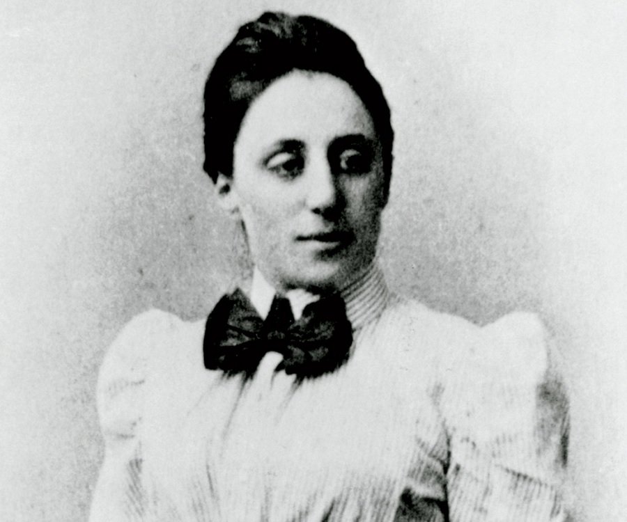
A true revolutionary in the field of theoretical physics and abstract algebra, Amelie Emmy Noether was a German-born inspiration thanks to her perseverance and passion for research. Instead of teaching French and English to schoolgirls, Emmy pursued the study of mathematics at the University of Erlangen. She then taught under a man’s name and without pay because she was a women.  During her exploration of the mathematics behind Einstein’s general relativity alongside renowned scientists like Hilbert and Klein, she discovered the fundamentals of conserved quantities such as energy and momentum under symmetric invariance of their respective quantities: time and homogeneity of space. She built the bridge between conservation and symmetry in nature, and although Noether’s Theorem is fundamental to our understanding of nature’s conservation laws, Emmy has received undeservedly small recognition throughout the last century.

Claudine Hermann – Helene Bresson

Claudine-HermannClaudine Hermann is a French physicist and Emeritus Professor at the École Polytechnique in Paris. Her work, on physics of solids (mainly on photo-emission of polarized electrons and near-field optics), led to her becoming the first female professor at this prestigious school. Aside from her work in Physics, Claudine studied and wrote about female scientists’ situation in Europe and the influence of both parents’ works on their daughter’s professional choices. Claudine wishes to give girls “other examples than the unreachable Marie Curie”. She is the founder of the Women and Sciences association and represented it at the European Commission to promote gender equality in Science and to help women accessing scientific knowledge. Claudine is also the president of the European Platform of Women Scientists which represents hundreds of associations and more than 12,000 female scientists.

Katherine Johnson – Sally Woodhouse

26646856911_ca242812ee_o_1
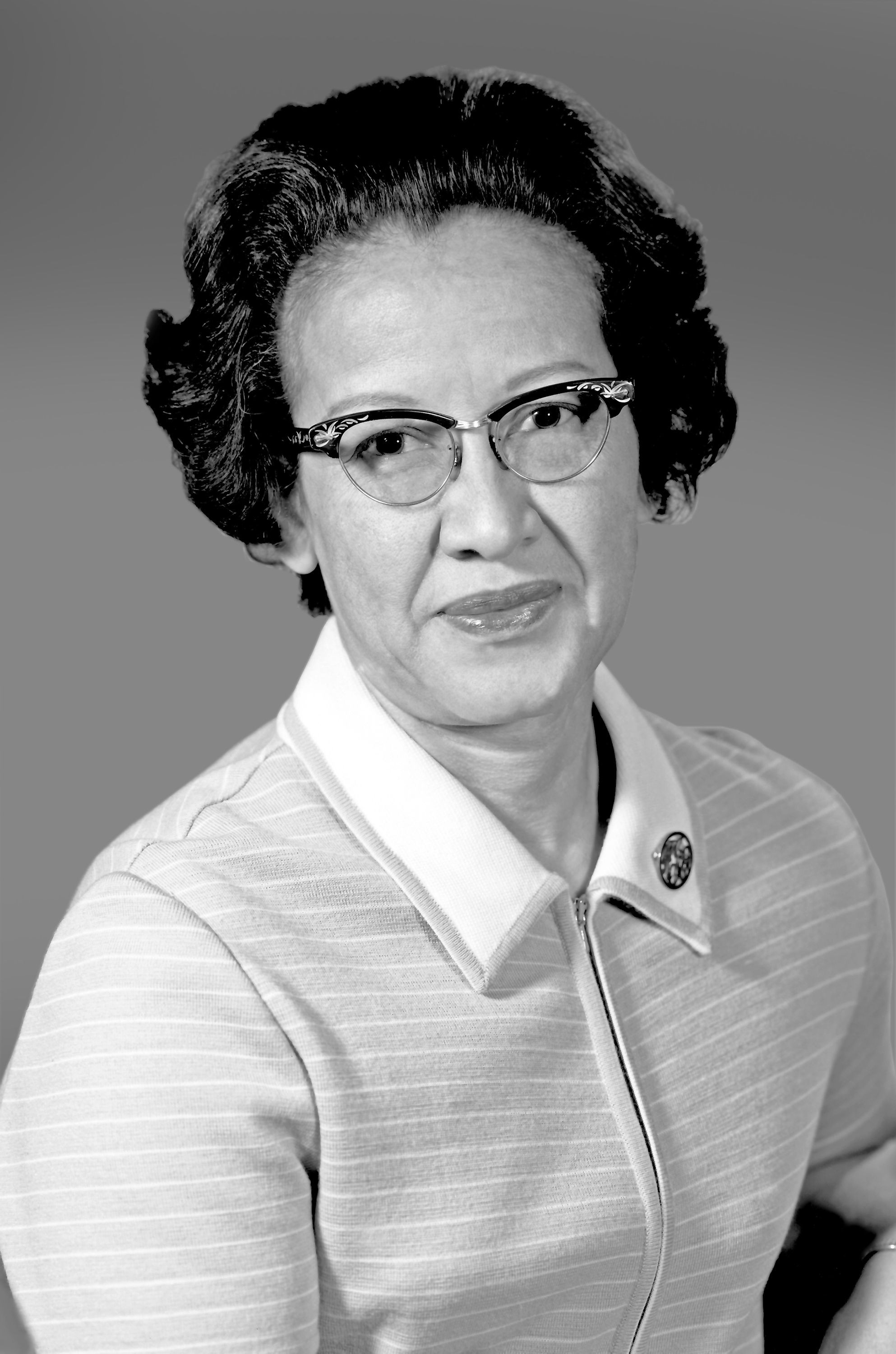
For most people being handpicked to be one of three students to integrate West Virginia’s graduate schools would probably be the most notable life achievements. However for Katherine Johnson’s this was just the start of a remarkable list of accomplishments. In 1952 Johnson joined the all-black West Area Computing section at NACA (to become NASA in 1958). Acting as a computer, Johnson analysed flight test data, provided maths for engineering lectures and worked on the trajectory for America’s first human space flight.

She became the first woman to receive an author credit on a Flight Research Division report in 1960 and went on to author or co-author 26 research reports. Johnson is perhaps best known (in part due to the excellent feel good film Hidden Figures) for her work on the flight trajectory for John Glenn’s 1962 orbital mission.

katherine_johnson_obama

She was required to check the calculations of NASA’s IBM computer and Glenn is reported to have asked for her to personally check the coordinates.

“GET THE GIRL TO CHECK THE NUMBERS… IF SHE SAYS THE NUMBERS ARE GOOD, I’M READY TO GO.”

Katherine was also involved in calculations for the Apollo missions trajectories, including Apollo 11. In 2015 she was presented with the Presidential Medal of Freedom by Barack Obama.

Marie Tharp – Caroline Dunning

World War II was an important period in terms of scientific advance. In addition, it enabled more women to be trained in professions such as geology, at a time when very few women were in earth sciences. One such woman was Marie Tharp. Following the advancement of sonar technology during WWII, in the early 1950s, ships travelled across the Atlantic Ocean recording ocean depth. maria-tharp-ocean
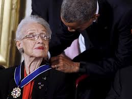
Women however were not allowed on such ships, thus Marie Tharp was stationed in the lab, checking and plotting the data. Her drawings showed the presence of the North Atlantic Ridge, with a deep V-shaped notch that ran the length of the mountain range, indicating the presence of a rift valley, where magma emerges to form new crust. At this time the theory of plate tectonics was seen as ridiculous. Her supervisor initially dismissed her results as ‘girl talk’ and forced her to redo them. The same results were found. Her work led to the acceptance of the theory of plate tectonics and continental drift.

Ada Lovelace – Dominic Jones

ada-lovelace-20825279-1-402Ada Lovelace was a 19th century Mathematician popularly referred to as the “first computer programmer”. She was the translator of “Sketch of the Analytical Engine, with Notes from the Translator”, (said “notes” tripling the length of the document and comprising its most striking insights) one of the documents critical to the development of modern computer programming. She was one of the few people to understand and even fewer who were able to develop for the machine. That she had such incredible insight into a machine which didn’t even exist yet, but which would go on to become so ubiquitous is amazing!

Drs. Jenni Evans, Sukyoung Lee, and Yvette Richardson – Michael Johnston

Leading Scientists at Penn State University, Drs. Jenni Evans, Sukyoung Lee, and Yvette Richardson serve as role models for students in STEM subjects. The three professors are active in linking their research interests to not only education but also science communication, and government policy. Between them, they highlight some of the many avenues a career in STEM can lead to. Whether its authoring a widely used textbook, leading advisory panels, or challenging students throughout their time in higher education – these leaders never cease to be an inspiration.


A week at COP23

From the 6th -17th of November the UNFCCC’s (United Nation Framework Convention on Climate Change) annual meeting or “Conference of the Parties” – COP took place. This year was COP23 and was hosted by Bonn in the UN’s world conference centre with Fiji taking the presidency.

IMG_20171106_123155780

Heading into the Bonn Zone on the first day of the COP. The Bonn Zone was the part of the conference for NGO stands and side events.

As part of the Walker Institutes Climate Action Studio another SCENARIO PhD and I attended the first week of the COP while students back in Reading participated remotely via the UNFCCC’s YouTube channel and through interviews with other participants of the COP.

There are many different components to the COP, it is primarily the meeting of a number of different international Climate agreements with lots of work currently being done on the implementation on the Paris Agreement. However it is also a space where many different civil society groups doing work connected to or impacted by climate change come together, to make connections with other NGOs as well as governments. This is done in an official capacity within the “exhibition zone” of the conference and with a vast array of side events taking place throughout the two weeks. Outside of these official events there are also many demonstrations both inside and outside of the conference space.

Demonstrations in the Bonn Zone

As an observer I was able to watch some of the official negotiations. On the Wednesday I attended the SBSTA (Subsidiary Body for Scientific and Technological Advice) informal consultation on research and systematic observations. It was an illuminating experience to see the negotiation process in action. At times it was frustrating to see how picky it feels like the negotiation teams can be, however over the week I did have a newfound appreciation for the complexity of the issues that are having to be resolved. This meeting was based on writing a short summary of the IPCC report and other scientific reports used by the COP, and so was less politically charged than a lot of the other meetings. However this didn’t stop an unexpected amount of debate over whether to include examples such as carbon-dioxide concentrations.

One of the most useful ways to learn about the COP was by talking to the different people and groups who we met at COP. It was interesting to see the different angles with which people were approaching the COP. From researchers who were observing the political process, to environmental and human rights NGO’s trying to get governments to engage with issues that they’re working on.

Interviewing other COP participants at the Walker Institutes stand

A particular highlight was the ex-leader of the Green Party Natalie Bennett, she spoke with us and the students back in Reading about a wide range of topics, from women’s involvement in the climate movement to discussing my PhD.

Kelly Stone from Action Aid provided a great insight into how charities operate at the COP. She spoke of making connections with other charities, often there are areas of overlap between their work but on other issues they had diverging opinions. However these differences have to be put aside to make progress on their shared interests. Kelly also discussed how it always amazes her that people are surprised that everyone who attends COP does not agree on everything, “we’re not deciding if climate change is real”. The issues being dealt with at the COP are complex dealing with human rights, economics, technology as well as climate change. Often serious compromises have to be made and this must be done by reaching a consensus between all 197 Parties to the UNFCCC.

To read more about the student experience of COP and summaries of specific talks and interviews you can view the COP CAS blog here. You can also read about last years COP on this blog here.

Clockwise from top left: The opening on the evening of Monday 6th November showed Fiji leaving its own mark as the President of the conference. The Norwegian Pavilion had a real Scandi feel, while the Fiji Pavilion transported visitors to a tropical island.


New Forecast Model Provides First Global Scale Seasonal River Flow Forecasts

new_web_figure2_rivernetwork

Over the past ~decade, extended-range forecasts of river flow have begun to emerge around the globe, combining meteorological forecasts with hydrological models to provide seasonal hydro-meteorological outlooks. Seasonal forecasts of river flow could be useful in providing early indications of potential floods and droughts; information that could be of benefit for disaster risk reduction, resilience and humanitarian aid, alongside applications in agriculture and water resource management.

While seasonal river flow forecasting systems exist for some regions around the world, such as the U.S., Australia, Africa and Europe, the forecasts are not always accessible, and forecasts in other regions and at the global scale are few and far between.  In order to gain a global overview of the upcoming hydrological situation, other information tends to be used – for example historical probabilities based on past conditions, or seasonal forecasts of precipitation. However, precipitation forecasts may not be the best indicator of floodiness, as the link between precipitation and floodiness is non-linear. A recent paper by Coughlan-de-Perez et al (2017), “should seasonal rainfall forecasts be used for flood preparedness?”, states:

“Ultimately, the most informative forecasts of flood hazard at the seasonal scale are streamflow forecasts using hydrological models calibrated for individual river basins. While this is more computationally and resource intensive, better forecasts of seasonal flood risk could be of immense use to the disaster preparedness community.”

twitter_screenshotOver the past months, researchers in the Water@Reading* research group have been working with the European Centre for Medium-Range Weather Forecasts (ECMWF), to set up a new global scale hydro-meteorological seasonal forecasting system. Last week, on 10th November 2017, the new forecasting system was officially launched as an addition to the Global Flood Awareness System (GloFAS). GloFAS is co-developed by ECMWF and the European Commission’s Joint Research Centre (JRC), as part of the Copernicus Emergency Management Services, and provides flood forecasts for the entire globe up to 30 days in advance. Now, GloFAS also provides seasonal river flow outlooks for the global river network, out to 4 months ahead – meaning that for the first time, operational seasonal river flow forecasts exist at the global scale – providing globally consistent forecasts, and forecasts for countries and regions where no other forecasts are available.

The new seasonal outlook is produced by forcing the Lisflood hydrological river routing model with surface and sub-surface runoff from SEAS5, the latest version of ECMWF’s seasonal forecasting system, (also launched last week), which consists of 51 ensemble members at ~35km horizontal resolution. Lisflood simulates the groundwater and routing processes, producing a probabilistic forecast of river flow at 0.1o horizontal resolution (~10km, the resolution of Lisflood) out to four months, initialised using the latest ERA-5 model reanalysis.

The seasonal outlook is displayed as three new layers in the GloFAS web interface, which is publicly (and freely) available at www.globalfloods.eu. The first of these gives a global overview of the maximum probability of unusually high or low river flow (defined as flow exceeding the 80th or falling below the 20th percentile of the model climatology), during the 4-month forecast horizon, in each of the 306 major world river basins used in GloFAS-Seasonal.

new_web_figure1_basins
The new GloFAS Seasonal Outlook Basin Overview and River Network Layers.

The second layer provides further sub-basin-scale detail, by displaying the global river network (all pixels with an upstream area >1500km2), again coloured according to the maximum probability of unusually high or low river flow during the 4-month forecast horizon. In the third layer, reporting points with global coverage are displayed, where more forecast information is available. At these points, an ensemble hydrograph is provided showing the 4-month forecast of river flow, with thresholds for comparison of the forecast to typical or extreme conditions based on the model climatology. Also displayed is a persistence diagram showing the weekly probability of exceedance for the current and previous three forecasts.

blog_screenshot
The new GloFAS Seasonal Outlook showing the river network and reporting points providing hydrographs and persistence diagrams.

Over the coming months, an evaluation of the system will be completed – for now, users are advised to evaluate the forecasts for their particular application. We welcome any feedback on the forecast visualisations and skill – feel free to contact me at the email address below!

To find out more, you can see the University’s press release here, further information on SEAS5 here, and the user information on the seasonal outlook GloFAS layers here.

*Water@Reading is “a vibrant cross-faculty centre of research excellence at the University of Reading, delivering world class knowledge in water science, policy and societal impacts for the UK and internationally.”

Full list of collaborators: 

Rebecca Emerton1,2, Ervin Zsoter1,2, Louise Arnal1,2, Prof. Hannah Cloke1, Dr. Liz Stephens1, Dr. Florian Pappenberger2, Prof. Christel Prudhomme2, Dr Peter Salamon3, Davide Muraro3, Gabriele Mantovani3

1 University of Reading
2 ECMWF
3 European Commission JRC

Contact: r.e.emerton@pgr.reading.ac.uk

Future of Cumulus Parametrization conference, Delft, July 10-14, 2017

Email: m.muetzelfeldt@pgr.reading.ac.uk

For a small city, Delft punches above its weight. It is famous for many things, including its celebrated Delftware (Figure 1). It was also the birthplace of one of the Dutch masters, Johannes Vermeer, who coincidentally painted some fine cityscapes with cumulus clouds in them (Figure 2). There is a university of technology with some impressive architecture (Figure 3). It holds the dubious honour of being the location of the first assassination using a pistol (or so we were told by our tour guide), when William of Orange was shot in 1584. To this list, it can now add hosting a one-week conference on the future of cumulus parametrization, and hopefully bringing about more of these conferences in the future.

Delftware_display

Figure 1: Delftware.

Vermeer-view-of-delft

Figure 2: Delft with canopy of cumulus clouds. By Johannes Vermeer, 1661.

Delft_AULA

Figure 3: AULA conference centre at Delft University of Technology – where we were based for the duration of the conference.

So what is a cumulus parametrization scheme? The key idea is as follows. Numerical weather and climate models work by splitting the atmosphere into a grid, with a corresponding grid length representing the length of each of the grid cells. By solving equations that govern how the wind, pressure and heating interact, models can then be used to predict what the weather will be like days in advance in the case of weather modelling. Or a model can predict how the climate will react to any forcings over longer timescales. However, any phenomena that are substantially smaller than this grid scale will not be “seen” by the models. For example, a large cumulonimbus cloud may have a horizontal extent of around 2km, whereas individual grid cells could be 50km in the case of a climate model. A cumulonimbus cloud will therefore not be explicitly modelled, but it will still have an effect on the grid cell in which it is located – in terms of how much heating and moistening it produces at different levels. To capture this effect, the clouds are parametrized, that is, the vertical profile of the heating and moistening due to the clouds are calculated based on the conditions in the grid cell, and this then affects the grid-scale values of these variables. A similar idea applies for shallow cumulus clouds, such as the cumulus humilis in Vermeer’s painting (Figure 2), or present-day Delft (Figure 3).

These cumulus parametrization schemes are a large source of uncertainty in current weather and climate models. The conference was aimed at bringing together the community of modellers working on these schemes, and working out which might be the best directions to go in to improve these schemes, and consequently weather and climate models.

Each day was a mixture of listening to presentations, looking at posters and breakout discussion groups in the afternoon, as well as plenty of time for coffee and meeting new people. The presentations covered a lot of ground: from presenting work on state-of-the-art parametrization schemes, to looking at how the schemes perform in operational models, to focusing on one small aspect of a scheme and modelling how that behaves in a high resolution model (50m resolution) that can explicitly model individual clouds. The posters were a great chance to see the in-depth work that had been done, and to talk to and exchange ideas with other scientists.

Certain ideas for improving the parametrization schemes resurfaced repeatedly. The need for scale-awareness, where the response of the parametrization scheme takes into account the model resolution, was discussed. One idea for doing this was the use of stochastic schemes to represent the uncertainty of the number of clouds in a given grid cell. The concept of memory also cropped up – where the scheme remembers if it had been active at a given grid cell in a previous point in time. This also ties into the idea of transitions between cloud regimes, e.g. when a stratocumulus layer splits up into individual cumulus clouds. Many other, sometimes esoteric, concepts were discussed, such as the role of cold pools, how much tuning of climate models is desirable and acceptable, how we should test our schemes, and what the process of developing the schemes should look like.

In the breakout groups, everyone was encouraged to contribute, which made for an inclusive atmosphere in which all points of view were taken on board. Some of the key points of agreement from these were that it was a good idea to have these conferences, and we should do it more often! Hopefully, in two years’ time, another PhD student will write a post on how the next meeting has gone. We also agreed that it would be beneficial to be able to share data from our different high resolution runs, as well as to be able to compare code for the different schemes.

The conference provided a picture of what the current thinking on cumulus parametrization is, as well as which directions people think are promising for the future. It also provided a means for the community to come together and discuss ideas for how to improve these schemes, and how to collaborate more closely with future projects such as ParaCon and HD(CP)2.

RMetS Impact of Science Conference 2017.

Email – j.f.talib@pgr.reading.ac.uk

“We aim to help people make better decisions than they would if we weren’t here”

Rob Varley CEO of Met Office

This week PhD students from the University of Reading attended the Royal Meteorological Society Impact of Science Conference for Students and Early Career Scientists. Approximately eighty scientists from across the UK and beyond gathered at the UK Met Office to learn new science, share their own work, and develop new communication skills.

image4

Across the two days students presented their work in either a poster or oral format. Jonathan Beverley, Lewis Blunn and I presented posters on our work, whilst Kaja Milczewska, Adam Bateson, Bethan Harris, Armenia Franco-Diaz and Sally Woodhouse gave oral presentations. Honourable mentions for their presentations were given to Bethan Harris and Sally Woodhouse who presented work on the energetics of atmospheric water vapour diffusion and the representation of mass transport over the Arctic in climate models (respectively). Both were invited to write an article for RMetS Weather Magazine (watch this space). Congratulations also to Jonathan Beverley for winning the conference’s photo competition!

IMG_3055
Jonathan Beverley’s Winning Photo.

Alongside student presentations, two keynote speaker sessions took place, with the latter of these sessions titled Science Communication: Lessons from the past, learning for future impact. Speakers in this session included Prof. Ellie Highwood (Professor of Climate Physics and Dean for Diversity and Inclusion at University of Reading), Chris Huhne (Co-chair of ET-index and former Secretary of State for Energy and Climate Change), Leo Hickman (editor for Carbon Brief) and Dr Amanda Maycock (NERC Independent Research Fellow and Associate Professor in Climate Dynamics, University of Leeds). Having a diverse range of speakers encouraged thought-provoking discussion and raised issues in science communication from many angles.

Prof. Ellie Highwood opened the session challenging us all to step beyond the typical methods of scientific communication. Try presenting your science without plots. Try presenting your work with no slides at all! You could step beyond the boundaries even more by creating interesting props (for example, the notorious climate change blanket). Next up Chris Huhne and Leo Hickman gave an overview of the political and media interactions with climate change science (respectively). The Brexit referendum, Trump’s withdrawal from the Paris Accord and the rise of the phrase “fake news” are some of the issues in a society “where trust in the experts is falling”. Finally, Dr Amanda Maycock presented a broad overview of influential science communicators from the past few centuries. Is science relying too heavily on celebrities for successful communication? Should the research community put more effort into scientific outreach?

Communication and collaboration became the two overarching themes of the conference, and conferences such as this one are a valuable way to develop these skills. Thank you to the Royal Meteorology Society and UK Met Office for hosting the conference and good luck to all the young scientists that we met over the two days.

#RMetSImpact

DEkAxGgXkAAmaWE.jpg large

Also thank you to NCAS for funding my conference registration and to all those who provided photos for this post.