Weather – The Social Metwork

Preparing for the assimilation of future ocean-current measurements

November 29, 2024The Social MetworkLeave a comment

By Laura Risley

Ocean data assimilation (DA) is vital. Firstly, it is essential to improving forecasts of ocean variables. Not only that, the interaction between the ocean and atmosphere is key to numerical weather prediction (NWP) as coupled ocean-atmosphere DA schemes are used operationally.

At present, observations of the ocean currents are not assimilated operationally. This is all set to change, as satellites are being proposed to measure these ocean currents directly. Unfortunately, the operational DA systems are not yet equipped to handle these observations due to some of the assumptions made about the velocities. In my work, we propose the use of alternative velocity variables to prepare for these future ocean current measurements. These will reduce the number of assumptions made about the velocities and is expected to improve the NWP forecasts.

What is DA?

DA combines observations and a numerical model to give a best estimate of the state of our system – which we call our analysis. This will lead to a better forecast. To quote my lunchtime seminar ‘Everything is better with DA!’.

Our model state usually comes from a prior estimate which we refer to as the background. A key component of data assimilation is that the errors present in both sets of data are taken into consideration. These uncertainties are represented by covariance matrices.

I am particularly interested in variational data assimilation, which formulates the DA problem into a least squares problem. Within variational data assimilation the analysis is performed with a set of variables that differ from the original model variables, called the control variables. After the analysis is found in this new control space, there is a transformation back to the model space. What is the purpose of this transformation? The control variables are chosen such that they can be assumed approximately uncorrelated, reducing the complexity of the data assimilation problem.

Velocity variables in the ocean

My work is focused on the treatment of the velocities in NEMOVAR. This is the data assimilation software used by the NEMO ocean model, used operationally at the Met Office and ECMWF. In NEMOVAR the velocities are transformed to their unbalanced components, and these are then used as control variables. The unbalanced components of the velocities are highly correlated, therefore contradicting the assumption made about control variables. This would result in suboptimal assimilation of future surface current measurements – therefore we seek alternative velocity control variables.

The alternative velocity control variables we propose for NEMOVAR are unbalanced streamfunction and velocity potential. This would involve transforming the current control variables, the unbalanced velocities, to these alternative variables using Helmholtz Theorem. This splits a velocity field into its nondivergent (streamfunction) and irrotational (velocity potential) parts. These parts have been suggested by Daley (1993) as more suitable control variables than the velocities themselves.

Numerical Implications of alternative variables

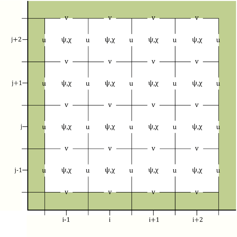
We have performed the transformation to these proposed control variables using the shallow water equations (SWEs) on a 𝛽-plane. To do so we discretised the variables on the Arakawa-C grid. The traditional placement of streamfunction on this grid causes issues with the boundary conditions. Therefore, Li et al. (2006) proposed placing streamfunction in the centre of the grid, as shown in Figure 1. This circumvents the need to impose explicit boundary conditions on streamfunction. However, using this grid configuration leads to numerical issues when transforming from the unbalanced velocities to unbalanced streamfunction and velocity potential. We have analysed these theoretically and here we show some numerical results.

Figure 1: The left figure shows the traditional Arakawa-C configuration (Lynch (1989), Watterson (2001)) whereby streamfunction is in the corner of each grid cell. The right figure shows the Arakawa-C configuration proposed by Li et al. (2006) where streamfunction is in the centre of the grid cell. The green shaded region represents land.

Issue 1: The checkerboard effect

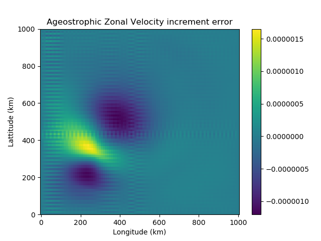
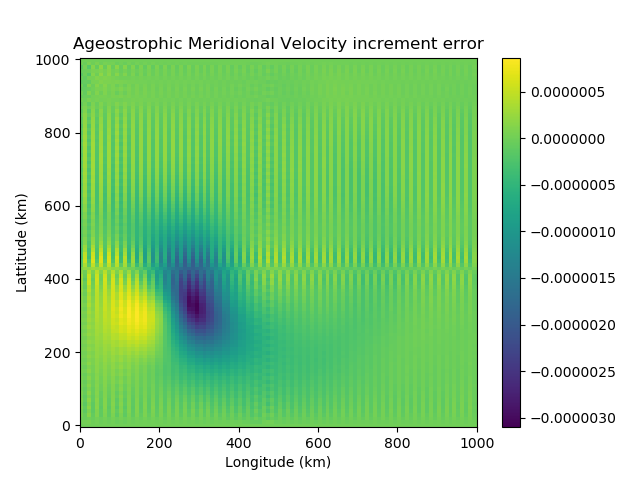
The transformation from the unbalanced velocities to unbalanced streamfunction and velocity potential involves averaging derivatives, due to the location of streamfunction in the grid cell. This process causes a checkerboard effect – whereby we have numerical noise entering the variable fields due to a loss of information. This is clear to see numerically using the SWEs. We use the shallow water model to generate a velocity field. This is transformed to its unbalanced components and then to unbalanced streamfunction and velocity potential. Using Helmholtz Theorem, the unbalanced velocities are reconstructed. Figure 2 shows the checkboard effect clearly in the velocity error.

Figure 2: The difference between the original ageostrophic velocity increments, calculated using the SWEs, and the reconstructed ageostrophic velocity increments. These are reconstructed using Helmholtz Theorem, from the ageostrophic streamfunction and velocity potential increments. On the left we have the zonal velocity increment error and on the right the meridional velocity increment error.

Issue 2: Challenges in satisfying the Helmholtz Theorem

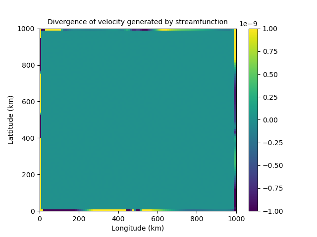
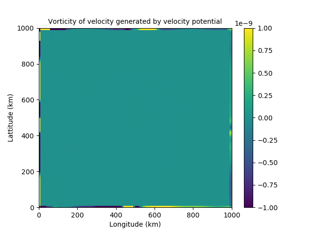
Helmholtz theorem splits the velocity into its nondivergent and irrotational components. We discovered that although streamfunction should be nondivergent and velocity potential should be irrotational, this is not the case at the boundaries, as can be seen in figure 3. This implies the proposed control variables are able to influence each other on the boundary. This would lead to them being strongly coupled and therefore correlated near the boundaries. This directly conflicts the assumption made that our control variables are uncorrelated.

Figure 3: Issues with Helmholtz Theorem near the boundaries. The left shows the divergence of the velocity field generated by streamfunction. The right shows the vorticity of the velocity field generated by velocity potential.

Overall, in my work we propose the use of alternative velocity control variables in NEMOVAR, namely unbalanced streamfunction and velocity potential. The use of these variables however leads to several numerical issues that we have identified and discussed. A paper on this work is in preparation, where we discuss some of the potential solutions. Our next work will further this investigation to a more complex domain and assess our proposed control variables in assimilation experiments.

References:

Daley, R. (1993) Atmospheric data analysis. No. 2. Cambridge university press.

Li, Z., Chao, Y. and McWilliams, J. C. (2006) Computation of the streamfunction and velocity potential for limited and irregular domains. Monthly weather review, 134, 3384–3394.

Lynch, P. (1989) Partitioning the wind in a limited domain. Monthly weather review, 117, 1492–1500.

Watterson, I. (2001) Decomposition of global ocean currents using a simple iterative method. Journal of Atmospheric and Oceanic Technology, 18, 691–703

Nature vs Nurture in Convective-Scale Ensemble Spread

November 8, 2024The Social MetworkLeave a comment

By Adam Gainford

Quantifying the uncertainty of upcoming weather is now a common procedure thanks to the widespread use of ensemble forecasting. Unlike deterministic forecasts, which show only a single realisation of the upcoming weather, ensemble forecasts predict a range of possible scenarios given the current knowledge of the atmospheric state. This approach allows forecasters to estimate the likelihood of upcoming weather events by simply looking at the frequency of event occurrence within all ensemble members. Additionally, by sampling a greater range of events, this approach highlights plausible worst-case scenarios, which is of particular interest for forecasts of extreme weather. Understanding the realistic range of outcomes is crucial for forecasters to provide informed guidance, and helps us avoid the kind of costly and embarrassing mistakes that are commonly associated with the forecast of “The Great Storm of 1987”*.

To have trust that our ensembles are providing an appropriate range of outputs, we need some method of verifying ensemble spread. We do this by calculating the spread-skill relationship, which essentially just compares the difference between member values to the skill of the ensemble as a whole. If the spread-skill relationship is appropriate, spread and skill scores should be comparable when averaged over many forecasts. If the ensemble shows a tendency to produce larger spread scores than skill scores, there is too much spread and not enough confidence in the ensemble given its accuracy: i.e., the ensemble is overspread. Conversely, if spread scores are smaller than skill scores, the ensemble is too confident and is underspread.

Figure 1: Postage stamp plots showing three-hourly precipitation accumulation valid for 2023-07-08 09Z at leadtime T+15 h. There is reasonable spread within both the frontal rain band effecting areas of SW England and Wales, and the convective features ahead of this front.

My PhD work has focussed on understanding the spread-skill relationship in convective-scale ensembles. Unlike medium range ensembles that are used to estimate the uncertainty of synoptic-scale weather at daily-to-weekly leadtimes, convective-scale ensembles quantify the uncertainty of smaller-scale weather at hourly-to-daily leadtimes. To do this, convective-scale ensembles must be run at higher resolutions than medium-range ensembles, with grid spacings smaller than 4 km. These higher resolutions allows the ensemble to explicitly represent convective storms, which has been repeatedly shown to produce more accurate forecasts compared coarser-resolution forecasts that must instead rely on convective parametrizations. However, running models at such high resolutions is too computationally expensive to be done over the entire Earth, so they are typically nested inside a lower-resolution “parent” ensemble which provides initial and boundary conditions. Despite this, researchers often report that convective-scale ensembles are underspread, and the range of outputs is too narrow given the ensemble skill. This is corroborated by operational forecasters, who report that the ensemble members often stay too close to the unperturbed control member.

To provide the necessary context for understanding the underspread problem, many studies have examined the different sources and behaviours of spread within convective-scale ensembles. In general, spread can be produced through three different mechanisms: firstly, through differences in each member’s initial conditions; secondly, through differences in the lateral boundary conditions provided to each member; and thirdly, through the different internal processes used to evolve the state. This last source is really the combination of many different model-specific factors (e.g., stochastic physics schemes, random parameter schemes etc.), but for our purposes this represents the ways in which the convective-scale ensemble produces its own spread. This contrasts with the other two sources of spread, which are directly linked to the spread of the parent ensemble.

The evolution of each of these three spread sources is shown in Fig. 2. At the start of a forecast, the ensemble spread is entirely dictated by differences in the initial conditions provided to each ensemble member. As we integrate forward in time, though, this initial information is removed from the domain by the prevailing winds and replaced by information arriving through the boundaries. At the same time, internal model processes start spinning up additional detail within each ensemble member. For a UK-sized domain, it takes roughly 12 hours for the initial information to have fully left the domain, though this is of course highly dependent on the strength of the prevailing winds. After this time, spread in the ensemble is partitioned between internal processes and boundary condition differences.

*Figure 2: Attribution of spread within a convective-scale ensemble by leadtime.*

While the exact partitioning in this schematic shouldn’t be taken too literally, it does highlight the important role that the parent ensemble plays in determining spread in the child ensemble. Most studies which try to improve spread target the child ensemble itself, but this schematic shows that these improvements may have quite a limited impact. After all, if the spread of information arriving from the parent ensemble is not sufficient, this may mask or even overwhelm any improvements introduced to the child ensemble.

However, there are situations where we might expect internal processes to show a more dominant spread contribution. Forecasts of convective storms, for instance, typically show larger spread than forecasts of other types of weather, and are driven more by local processes than larger-scale, external factors.

This is where our “nature” and “nurture” analogy becomes relevant. Given the similarities of this relationship to the common parent-child theory in behavioural psychology, we thought it would be a fun and useful gimmick to also use this terminology here. So, in the “nature” scenario, each child member shows large similarity to the corresponding parent member, which is due to the dominating influence of genetics (initial and boundary conditions). Conversely, in the “nurture” scenario, spread in the child ensemble is produced more by its response to the environment (internal processes), and as such, we see larger differences between each parent-child pair.

While the nature and nurture attribution is well understood for most variables, few studies have examined the parent-child relationship for precipitation patterns, which are an important output for guidance production and require the use of neighbourhood-based metrics for robust evaluation. Given that this is already quite a long post, I won’t go into too much detail of our results looking at nature vs nurture for precipitation patterns. Instead, I will give a quick summary of what we found:

Nurture provides a larger than average influence on the spread in two situations: during short leadtimes**, and when forecasting convective events driven by continental plume setups.

In the nurture scenarios, spread is consistently larger in the child ensemble than the parent ensemble.

In contrast to the nurture scenarios, nature provides larger than average spread at medium-to-long leadtimes and under mobile regimes, which is consistent with the boundary arguments mentioned previously.

Spread is very similar between the child and parent ensembles in the nurture scenarios.

If you would like to read more about this work, we will be submitting a draft to QJRMS very soon.

To conclude, if we want to improve the spread of precipitation patterns in convective-scale ensembles, we should direct more attention to the role of the driving ensemble. It is clear that the exact nesting configuration used has a strong impact on the quality of the spread. This factor is especially important to consider given recent experiments with hectometric-scale ensembles which are themselves nested within convective-scale ensembles. With multiple layers of nesting, the coupling between each ensemble layer is likely to be complex. Our study provides the foundation for investigating these complex interactions in more detail.

* This storm was actually well forecast by the Met Office. The infamous Michael Fish weather update in which he said there was no hurricane on the way was referring to a different system which indeed did not impact the UK. Nevertheless, this remains a good example of the importance of accurately predicting (and communicating) extreme weather events.

** While this appears to be inconsistent with Fig. 2, the ensemble we used does not solely take initial conditions from the driving ensemble. Instead, the ensemble uses a separate, high-resolution data assimilation scheme to the parent ensemble. Each ensemble is produced in a way which makes the influence of the data assimilation more influential to the spread than the initial condition perturbations.

The importance of anticyclonic synoptic eddies for atmospheric block persistence and forecasts

May 3, 2024The Social MetworkLeave a comment

Charlie Suitters – c.c.suitters@pgr.reading.ac.uk

The Beast from the East, the record-breaking winter warmth of February 2020, the Canadian heat dome of 2022…what do these three events have in common? Well, many things I’m sure, but most relevantly for this blog post is that they all coincided with the same phenomenon – atmospheric blocking.

So what exactly is a block? An atmospheric block is a persistent, large-scale, quasi-stationary high-pressure system sometimes found in the mid-latitudes. The prolonged subsidence associated with the high pressure suppresses cloud formation, therefore blocks are often associated with clear, sunny skies, calm winds, and temperature extremes. Their impacts can be diverse, including both extreme heat and extreme cold, drought, poor air quality, and increased energy demand (Kautz et al., 2022).

Despite the range of hazards that blocking can bring, we still do not fully understand the dynamics that cause a block to start, maintain itself, and decay (Woollings et al., 2018). In reality, many different mechanisms are at play, but the importance of each process can vary between location, season, and individual block events (Miller and Wang, 2022). One process that is known to be important is the interaction between blocks and smaller synoptic-scale transient eddies (Shutts, 1983; Yamazaki and Itoh, 2013). By studying a 43-year climatology of atmospheric blocks and their anticyclonic eddies (both defined by regions of anomalously high 500 hPa geopotential height), I have found that on average, longer blocks absorb more synoptic anticyclones, which “tops up their anticyclonicness” and allows them to persist longer (Fig. 1).

Figure 1: average number of anticyclonic eddies per block for the Euro-Atlantic (left) and North Pacific (right). Block persistence is defined as the quartiles (Q1, Q2, Q3) of all blocks in winter (blue) and summer (red). From Suitters et al. (2023).

It’s great that we now know this relationship, however it would be beneficial to know if these interactions are forecasted well. If they are not, it might explain our shortcomings in predicting the longevity of a block event (Ferranti et al., 2015). I explore this with a case study from March 2021 using ensemble forecasts from MOGREPS-G. Fortunately, this block in March 2021 was not associated with any severe weather, but it was still not forecasted well. In Figure 2, I show normalised errors in the strength, size, and location of the block, at the time of block onset, for each ensemble member from a range of different initialisation times. In these plots, a negative (positive) value means that the block was forecast to be too weak (strong) or too small (large), and the larger the error in the location, the further away the forecast block was from reality. In general, the onset of this block was forecast to be to be too weak and too small, though there was considerable spread within the ensemble (Fig. 2). Certainty in the forecast was only achieved at relatively small lead times.

Figure 2: Normalised errors in the intensity (left), area (centre), and location of the block’s centre of mass (right), at a validity time of 2021-03-14 12 UTC (the time of onset). Each ensemble member’s error from a particular initialisation time is shown by the grey dots, and the ensemble mean is shown in black. When Z, A, or L are zero, the forecast has a “perfect” replication for this metric of the block (when compared to ERA5 reanalysis).

Now for the interesting bit – what causes the uncertainty in forecasting of the onset this European blocking event? To examine this, I grouped forecast members from an initialisation time of 8 March 2021 according to their ability to replicate the real block: the entire MOGREPS-G mean, members that either have no block or a very small block (Group G), members that perform best (Group H), and members that predict area well, but have the block in the wrong location (Group I). Then, I take the mean geopotential height anomalies () at each time step in each group, and compare these fields between groups to see if I can find a source of forecast error.

This is shown as an animation in Fig. 3. The animation starts at the time of block onset, and goes back in time to selected validity times, as shown at the top of the figure. The domain of the plot also changes in each frame, gradually moving westwards across the Atlantic. By looking at the ERA5 (the “real”) evolution of the block, we see that the onset of the European block was the result of an anticyclonic transient eddy breaking off from an upstream blocking event over North America. However, none of the aforementioned groups of members accurately simulate this vortex shedding from the North American block. In most cases, the eddy leaving the North American block is either too weak or non-existent (as shown by the blue shading, representing that the forecast is much weaker than in ERA5), which resulted in a lack of Eastern Atlantic blocking altogether. Only the group that modelled the block well (Group H) had a sizeable eddy breaking off from the upstream block, but even in this case it was too weak (paler blue shading). Therefore, the uncertain block onset in this case is directly related to the way in which an anticyclonic eddy was forecast to travel (or not) across the Atlantic, from a pre-existing block upstream. This is interesting because the North American block itself was modelled well, yet the eddy that broke off it was not, which was vital for the onset of the Euro-Atlantic block.

To conclude, this is an important finding because it shows the need to accurately model synoptic-scale features in the medium range in order to accurately predict blocking. If these eddies are absent in a forecast, a block might not even form (as I have shown), and therefore potentially hazardous weather conditions would not be forecast until much shorter lead times. My work shows the role of anticyclonic eddies towards the persistence and forecasting of blocks, which until now had not be considered in detail.

References

Kautz, L., Martius, O., Pfahl, S., Pinto, J.G., Ramos, A.M., Sousa, P.M., and Woollings, T., 2022. “Atmospheric blocking and weather extremes over the Euro-Atlantic sector–a review.” Weather and climate dynamics, 3(1), pp305-336.

Miller, D.E. and Wang, Z., 2022. Northern Hemisphere winter blocking: differing onset mechanisms across regions. Journal of the Atmospheric Sciences, 79(5), pp.1291-1309.

Shutts, G.J., 1983. The propagation of eddies in diffluent jetstreams: Eddy vorticity forcing of ‘blocking’ flow fields. Quarterly Journal of the Royal Meteorological Society, 109(462), pp.737-761.

Suitters, C.C., Martínez-Alvarado, O., Hodges, K.I., Schiemann, R.K. and Ackerley, D., 2023. Transient anticyclonic eddies and their relationship to atmospheric block persistence. Weather and Climate Dynamics, 4(3), pp.683-700.

Woollings, T., Barriopedro, D., Methven, J., Son, S.W., Martius, O., Harvey, B., Sillmann, J., Lupo, A.R. and Seneviratne, S., 2018. Blocking and its response to climate change. Current climate change reports, 4, pp.287-300.

Yamazaki, A. and Itoh, H., 2013. Vortex–vortex interactions for the maintenance of blocking. Part I: The selective absorption mechanism and a case study. Journal of the Atmospheric Sciences, 70(3), pp.725-742.

How does plasma from the solar wind enter Earth’s magnetosphere?

February 23, 2018February 23, 2018Sarah Bentley1 Comment

Earth’s radiation belts are a hazardous environment for the satellites underpinning our everyday life. The behaviour of these high-energy particles, trapped by Earth’s magnetic field, is partly determined by the existence of plasma waves. These waves provide the mechanisms by which energy and momentum are transferred and particle populations physically moved around, and it’s some of these waves that I study in my PhD.

However, I’ve noticed that whenever I talk about my work, I rarely talk about where this plasma comes from. In schools it’s often taught that space is a vacuum, and while it is closer to a vacuum than anything we can make on Earth, there are enough particles to make it a dangerous environment. A significant amount of particles do escape from Earth’s ionosphere into the magnetosphere but in this post I’ll focus on material entering from the solar wind. This constant outflow of hot particles from the Sun is a plasma, a fluid where enough of the particles are ionised that the behaviour of the fluid is then dominated by electric and magnetic fields. Since the charged particles in a plasma interact with each other, with external electric and magnetic fields, and also generate more fields by moving and interacting, this makes for some weird and wonderful behaviour.

magnetosphere_diagram — Figure 1: The area of space dominated by Earth’s magnetic field (the magnetosphere) is shaped by the constant flow of the solar wind (a plasma predominantly composed of protons, electrons and alpha particles). Plasma inside the magnetosphere collects in specific areas; the radiation belts are particularly of interest as particles there pose a danger to satellites. **Credit:** NASA/Goddard/Aaron Kaas

When explaining my work to family or friends, I often describe Earth’s magnetic field as a shield to the solar wind. Because the solar wind is well ionised, it is highly conductive, and this means that approximately, the magnetic field is “frozen in” to the plasma. If the magnetic field changes, the plasma follows this change. Similarly, if the plasma flows somewhere, the magnetic field is dragged along with it. (This is known as Alfvén’s frozen in theorem – the amount of plasma in a volume parallel to the magnetic field line remains constant). And this is why the magnetosphere acts as shield to all this energy streaming out of the Sun – while the magnetic field embedded in the solar wind is topologically distinct from the magnetic field of the Earth, there is no plasma transfer across magnetic field lines, and it streams past our planet (although this dynamic pressure still compresses the plasma of the magnetosphere, giving it that typical asymmetric shape in Figure 1).

Of course, the question still remains of how the solar wind plasma enters the Earth’s magnetic field if such a shielding effect exists. You may have noticed in Figure 1 that there are gaps in the shield that the Earth’s dipole magnetic field presents to the solar wind; these are called the cusps, and at these locations the magnetic field connects to the solar wind. Here, plasma can travel along magnetic field lines and impact us on Earth.

But there’s also a more interesting phenomenon occurring – on a small enough scale (i.e. the very thin boundaries between two magnetic domains) the assumptions behind the frozen-in theorem break down, and then we start to see one of the processes that make the magnetosphere such a complex, fascinating and dynamic system to study. Say we have two regions of plasma with opposing orientation of the magnetic field. Then in a middle area these opposing field lines will suddenly snap to a new configuration, allowing them to peel off and away from this tightly packed central region. Figure 2 illustrates this process – you can see that after pushing red and blue field lines together, they suddenly jump to a new configuration. As well as changing the topology of the magnetic field, the plasma at the centre is energised and accelerated, shooting off along the magnetic field lines. Of course even this is a simplification; the whole process is somewhat more messy in reality and I for one don’t really understand how the field can suddenly “snap” to a new configuration.

Figure 2: Magnetic reconnection. Two magnetic domains of opposing orientation can undergo a process where the field line configuration suddenly resets. Instead of two distinct magnetic domains, some field lines are suddenly connected to both, and shoot outwards and away, as does the energised plasma.

In the Earth’s magnetosphere there are two main regions where this process is important (Figure 3). Firstly, at the nose of the magnetosphere. The dynamic pressure of the solar wind is compressing the solar wind plasma against the magnetospheric plasma, and when the interplanetary magnetic field is orientated downwards (i.e. opposite to the Earth’s dipole – about half the time) this reconnection can happen. At this point field lines that were solely connected to the Earth or in the solar wind are now connected to both, and plasma can flow along them.

magnetosphere_reconnection_sites — Figure 3: There are two main areas where reconnection happens in Earth’s magnetosphere. Opposing field lines can reconnect, allowing a continual dynamic cycle (the Dungey cycle) of field lines around the magnetosphere. Plasma can travel along these magnetic field lines freely. **Credits**: NASA/MMS (image) and NASA/Goddard Space Flight Center- Conceptual Image Lab (video)

Then, as the solar wind continues to rush outwards from the Sun, it drags these field lines along with it, past the Earth and into the tail of the magnetosphere. Eventually the build-up of these field lines reaches a critical point in the tail, and boom! Reconnection happens once more. You get a blast of energised plasma shooting along the magnetic field (this gives us the aurora) and the topology has rearranged to separate the magnetic fields of the Earth and solar wind; once more, they are distinct. These dipole field lines move around to the front of the Earth again, to begin this dramatic cycle once more.

Working out when and how these kind of processes take place is still an active area of research, let alone understanding exactly what we expect this new plasma to do when it arrives. If it doesn’t give us a beautiful show of the aurora, will it bounce around the radiation belts, trapped in the stronger magnetic fields near the Earth? Or if it’s not so high energy as that, will it settle in the cooler plasmasphere, to rotate with the Earth and be shaped as the magnetic field is distorted by solar wind variations? Right now I look out my window at a peaceful sunny day and find it incredible that such complicated and dynamic processes are continually happening so (relatively) nearby. It certainly makes space physics an interesting area of research.

RMetS Impact of Science Conference 2017.

July 14, 2017The Social Metwork1 Comment

Email – j.f.talib@pgr.reading.ac.uk

“We aim to help people make better decisions than they would if we weren’t here”

Rob Varley CEO of Met Office

This week PhD students from the University of Reading attended the Royal Meteorological Society Impact of Science Conference for Students and Early Career Scientists. Approximately eighty scientists from across the UK and beyond gathered at the UK Met Office to learn new science, share their own work, and develop new communication skills.

Across the two days students presented their work in either a poster or oral format. Jonathan Beverley, Lewis Blunn and I presented posters on our work, whilst Kaja Milczewska, Adam Bateson, Bethan Harris, Armenia Franco-Diaz and Sally Woodhouse gave oral presentations. Honourable mentions for their presentations were given to Bethan Harris and Sally Woodhouse who presented work on the energetics of atmospheric water vapour diffusion and the representation of mass transport over the Arctic in climate models (respectively). Both were invited to write an article for RMetS Weather Magazine (watch this space). Congratulations also to Jonathan Beverley for winning the conference’s photo competition!

Alongside student presentations, two keynote speaker sessions took place, with the latter of these sessions titled Science Communication: Lessons from the past, learning for future impact. Speakers in this session included Prof. Ellie Highwood (Professor of Climate Physics and Dean for Diversity and Inclusion at University of Reading), Chris Huhne (Co-chair of ET-index and former Secretary of State for Energy and Climate Change), Leo Hickman (editor for Carbon Brief) and Dr Amanda Maycock (NERC Independent Research Fellow and Associate Professor in Climate Dynamics, University of Leeds). Having a diverse range of speakers encouraged thought-provoking discussion and raised issues in science communication from many angles.

Prof. Ellie Highwood opened the session challenging us all to step beyond the typical methods of scientific communication. Try presenting your science without plots. Try presenting your work with no slides at all! You could step beyond the boundaries even more by creating interesting props (for example, the notorious climate change blanket). Next up Chris Huhne and Leo Hickman gave an overview of the political and media interactions with climate change science (respectively). The Brexit referendum, Trump’s withdrawal from the Paris Accord and the rise of the phrase “fake news” are some of the issues in a society “where trust in the experts is falling”. Finally, Dr Amanda Maycock presented a broad overview of influential science communicators from the past few centuries. Is science relying too heavily on celebrities for successful communication? Should the research community put more effort into scientific outreach?

Communication and collaboration became the two overarching themes of the conference, and conferences such as this one are a valuable way to develop these skills. Thank you to the Royal Meteorology Society and UK Met Office for hosting the conference and good luck to all the young scientists that we met over the two days.

#RMetSImpact

DEkAxGgXkAAmaWE.jpg large

Also thank you to NCAS for funding my conference registration and to all those who provided photos for this post.

The Influence of the Weather on Bird Migration

March 23, 2017David FlackLeave a comment

Email: d.l.a.flack@pgr.reading.ac.uk

As well as being a meteorologist, I am a bird watcher. This means I often combine meteorology and bird watching to see the impact of the weather on birds. Now that we are well into March my focus in bird watching turns to one thing – the migration.

March generally marks the time when the first summer migrants start arriving into the UK. Already this year we have had reports of Sand Martin, Wheatear, Garganey, Little Ringed Plover, White Wagtail, Osprey, Swallow, House Martin, Ring Ouzel and Whitethroat (up to 9 March), some of which are depicted below.

There are many people that consider the arrival dates of certain migratory species of birds and how this arrival date changes over many years. I do keep extensive records of the birds that I see (and thus arrival dates), but what interests me more are the odd days in the record, and the sightings of unusual birds and working out how they arrived at their destinations.

A good example of this can be found by looking at my first Swallow sighting of the year in Kent and East Sussex. Since I started bird watching in 2001 my first Swallow of the year has moved from around 10 April to between 26-March and 1 April. However in 2013 my first record was 15 April. Then in 2015 and 2016 I saw my first Swallow on 1 April and 27 March respectively (I was in Cheshire in 2014 in late March/early April).

So what happened; why were the Swallows late in Kent in 2013? Well, it all comes down to wind direction. The spring of 2013 was very chilly and along the east coast there were plenty of N/NE winds – this would have provided a head wind so the Swallows would preferentially not migrate up the east coast in those conditions but instead migrate up the west coast where there were southerlies.

So, the wind direction plays a key part in the migration of birds. If conditions are for a tailwind or very light winds the birds will migrate; otherwise they will stay put. However, headwinds can lead to some interesting phenomena associated with bird migration – ‘falls’.

A ‘fall’ occurs when there are a large number of migrants building up along the coastline at a departure point (so for the interest of UK bird watchers Northern France), as they cannot get to their destination. When the wind direction changes the birds will then migrate en masse and quite literally fall out of the sky.

It’s not all about the wind direction though; rain is also a key factor that bird watchers consider when looking at weather forecasts. Essentially, fronts and showers are great for bird watchers. On migration birds will often fly higher than they normally would. This means on a clear sunny day you could easily miss birds passing overhead as they are so high up. However, with the rain the birds will often fly lower, avoiding the in-cloud turbulence. For many of the summer migrants their food sources (insects) also fly lower in these conditions.

This means that a forecast of showers with a southerly wind is generally what I look for from mid-April onwards (particularly as an inland birder), as it means there is a good chance of migratory species turning up – also because then I can head out after work as the evenings are brighter. This is something that I did last year and ended up recording the first Sandwich Tern (photo below (not of the bird I saw)) of the year in Berkshire.

So in summary, it’s not as simple as just keeping an eye on the wind direction – there are other factors that can influence the birds’ migration and where they will end up. For more information about the impact of weather on bird sightings (considering both rare and common birds) check out my blog.

Share this:

Share this:

References

Share this:

Share this:

Share this:

Share this: