On 22nd and 23rd February, a group of students from the University of Reading visited the UK Met Office in Exeter to share our work and listen to talks from academics and Met Office employees. It was a great opportunity to discuss our work with other scientists from outside the university.
We arrived at the Met Office at 12 on the Wednesday. Once we had hung up our posters and had lunch, we listened to our first talk from Dale Barker, who is Deputy Director of Weather Science at the UK Met Office. He gave us an overview of the Met Office Academic Partnership (MOAP) and the variety of work that takes place within the partnership. The MOAP brings together the UK Met Office with the universities of Exeter, Reading, Leeds, and Oxford to collaborate on projects and share science. It aims to pull together world-class expertise in weather and climate science to tackle key problems in these areas, and to provide an environment to develop the science leaders of tomorrow. The next talk was from Prof. Nadine Unger from the University of Exeter who spoke about aerosol pollution and work she has been involved in with African nations to reduce health problems caused by pollution. Our very own Dr Clare Watt then spoke about space weather, focusing on the magnetosphere and the impact of ‘killer’ electrons. The final talk of the day was from Dr Steven Böing from the University of Leeds. He spoke about semi-Lagrangian cloud modelling and how it can be used to increase forecast accuracy.
The poster session then took place in the Street. A lot of useful discussions were had during this session (and over the whole two days) as we were able to share our work with each other and also with passing members of Met Office staff. I certainly realized some new things about my results and had ideas about future directions for my work.
On the second day we had a presentation on career opportunities within the scientific areas of the Met Office from Mo Mylne, who is Science Project and Planning Manager at the UK Met Office. This really highlighted the breadth of roles that are available at the national meteorological service. This was followed by a talk from Prof. Coralia Cartis from the University of Oxford who spoke about parameter estimation for climate modelling using optimization techniques. After this, we were taken on tours of the Met Office to see some of areas that scientists are involved in. We then had lunch and a final opportunity to discuss our posters before the event finished.
Overall, then, it was a very enjoyable event with a great variety of subjects covered by the talks. I found the use of optimization techniques for parameter estimation particularly interesting and I hope to incorporate some of the ideas into my own research. I feel I have personally learned a lot, both about my own results and new ideas to consider. Thank you to all at the Met Office who organized the event.
Forests play an important role in the global carbon cycle, removing large amounts of CO2 from the atmosphere and thus helping to mitigate the effect of human-induced climate change. The state of the global carbon cycle in the IPCC AR5 suggests that the land surface is the most uncertain component of the global carbon cycle. The response of ecosystem carbon uptake to land use change and disturbance (e.g. fire, felling, insect outbreak) is a large component of this uncertainty. Additionally, there is much disagreement on whether forests and terrestrial ecosystems will continue to remove the same proportion of CO2 from the atmosphere under future climate regimes. It is therefore important to improve our understanding of ecosystem carbon cycle processes in the context of a changing climate.
Here we focus on the effect on ecosystem carbon dynamics of disturbance from selective felling (thinning) at the Alice Holt research forest in Hampshire, UK. Thinning is a management practice used to improve ecosystem services or the quality of a final tree crop and is globally widespread. At Alice Holt a program of thinning was carried out in 2014 where one side of the forest was thinned and the other side left unmanaged. During thinning approximately 46% of trees were removed from the area of interest.
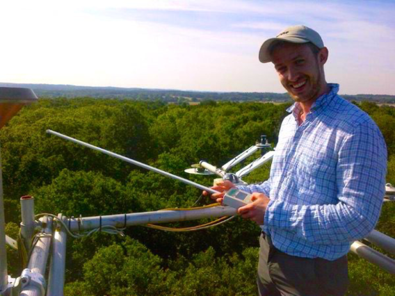
Figure 1: At the top of Alice Holt flux tower.
Using the technique of eddy-covariance at flux tower sites we can produce direct measurements of the carbon fluxes in a forest ecosystem. The flux tower at Alice Holt has been producing measurements since 1999 (Wilkinson et al., 2012), a view from the flux tower is shown in Figure 1. These measurements represent the Net Ecosystem Exchange of CO2 (NEE). The NEE is composed of both photosynthesis and respiration fluxes. The total amount of carbon removed from the atmosphere through photosynthesis is termed the Gross Primary Productivity (GPP). The Total Ecosystem Respiration (TER) is made up of autotrophic respiration (Ra) from plants and heterotrophic respiration (Rh) from soil microbes and other organisms incapable of photosynthesis. We then have, NEE = -GPP + TER, so that a negative NEE value represents removal of carbon from the atmosphere and a positive NEE value represents an input of carbon to the atmosphere. A schematic of these fluxes is shown in Figure 2.
Figure 2: Fluxes of carbon around a forest ecosystem.
The flux tower at Alice Holt is on the boundary between the thinned and unthinned forest. This allows us to partition the NEE observations between the two areas of forest using a flux footprint model (Wilkinson et al., 2016). We also conducted an extensive fieldwork campaign in 2015 to estimate the difference in structure between the thinned and unthinned forest. However, these observations are not enough alone to understand the effect of disturbance. We therefore also use mathematical models describing the carbon balance of our ecosystem, here we use the DALEC2 model of ecosystem carbon balance (Bloom and Williams, 2015). In order to find the best estimate for our system we use the mathematical technique of data assimilation in order to combine all our available observations with our prior model predictions. More infomation on the novel data assimilation techniques developed can be found in Pinnington et al., 2016. These techniques allow us to find two distinct parameter sets for the DALEC2 model corresponding to the thinned and unthinned forest. We can then inspect the model output for both areas of forest and attempt to further understand the effect of selective felling on ecosystem carbon dynamics.
Figure 3: Model predicted cumulative fluxes for 2015 after data assimilatiom. Solid line: NEE, dotted line: TER, dashed line: GPP. Orange: model prediction for thinned forest, blue: model prediction for unthinned forest. Shaded region: model uncertainty after assimilation (± 1 standard deviation).
In Figure 3 we show the cumulative fluxes for both the thinned and unthinned forest after disturbance in 2015. We would probably assume that removing 46% of the trees from the thinned section would reduce the amount of carbon uptake in comparison to the unthinned section. However, we can see that both forests removed a total of approximately 425 g C m-2 in 2015, despite the thinned forest having 46% of its trees removed in the previous year. From our best modelled predictions this unchanged carbon uptake is possible due to significant reductions in TER. So, even though the thinned forest has lower GPP, its net carbon uptake is similar to the unthinned forest. Our model suggests that GPP is a main driver for TER, therefore removing a large amount of trees has significantly reduced ecosystem respiration. This result is supported by other ecological studies (Heinemeyer et al., 2012, Högberg et al., 2001, Janssens et al., 2001). This has implications for future predictions of land surface carbon uptake and whether forests will continue to sequester atmospheric CO2 at similar rates, or if they will be limited by increased GPP leading to increased respiration.
References
Wilkinson, M. et al., 2012: Inter-annual variation of carbon uptake by a plantation oak woodland in south-eastern England. Biogeosciences, 9 (12), 5373–5389.
Wilkinson, M., et al., 2016: Effects of management thinning on CO2 exchange by a plantation oak woodland in south-eastern England. Biogeosciences, 13 (8), 2367–2378, doi: 10.5194/bg-13-2367-2016.
Bloom, A. A. and M. Williams, 2015: Constraining ecosystem carbon dynamics in a data-limited world: integrating ecological “common sense” in a model data fusion framework. Biogeosciences, 12 (5), 1299–1315, doi: 10.5194/bg-12-1299-2015.
Pinnington, E. M., et al., 2016: Investigating the role of prior and observation error correlations in improving a model forecast of forest carbon balance using four-dimensional variational data assimilation. Agricultural and Forest Meteorology, 228229, 299 – 314, doi: http://dx.doi.org/10.1016/j.agrformet.2016.07.006.
Heinemeyer, A., et al., 2012: Exploring the “overflow tap” theory: linking forest soil co2 fluxes and individual mycorrhizo- sphere components to photosynthesis. Biogeosciences, 9 (1), 79–95.
Högberg, P., et al., 2001: Large-scale forest girdling shows that current photosynthesis drives soil respiration. Nature, 411 (6839), 789–792.
Janssens, I. A., et al., 2001: Productivity overshadows temperature in determining soil and ecosystem respiration across european forests. Global Change Biology, 7 (3), 269–278, doi: 10.1046/j.1365-2486.2001.00412.x.
Gristey, J. J., J. C. Chiu, R. J. Gurney, S.-C. Han, and C. J. Morcrette (2017), Determination of global Earth outgoing radiation at high temporal resolution using a theoretical constellation of satellites, J. Geophys. Res. Atmos., 122, doi:10.1002/2016JD025514.
The surface of our planet has warmed at an unprecedented rate since the mid-19th century and there is no sign that the rate of warming is slowing down. The last three decades have all been successively warmer than any preceding decade since 1850, and 16 of the 17 warmest years on record have all occurred since 2001. The latest science now tells us that it is extremely likely that human influence has been the dominant cause of the observed warming1, mainly due to the release of carbon dioxide and other greenhouse gases into our atmosphere. These greenhouse gases trap heat energy that would otherwise escape to space, which disrupts the balance of energy flows at the top of the atmosphere (Fig. 1). The current value of the resulting energy imbalance is approximately 0.6 W m–2, which is more than 17 times larger than all of the energy consumed by humans2! In fact, observing the changes in these energy flows at the top of the atmosphere can help us to gauge how much the Earth is likely to warm in the future and, perhaps more importantly, observations with sufficient spatial coverage, frequency and accuracy can help us to understand the processes that are causing this warming.
Figure 1. The Earth’s top-of-atmosphere energy budget. In equilibrium, the incoming sunlight is balanced by the reflected sunlight and emitted heat energy. Greenhouse gases can reduce the emitted heat energy by trapping heat in the Earth system leading to an energy imbalance at the top of the atmosphere.
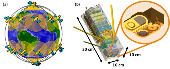
Observations of energy flows at the top of the atmosphere have traditionally been made by large and expensive satellites that may be similar in size to a large car3, making it impractical to launch multiple satellites at once. Although such observations have led to many advancements in climate science, the fundamental sampling restrictions from a limited number of satellites makes it impossible to fully resolve the variability in the energy flows at the top of atmosphere. Only recently, due to advancements in small satellite technology and sensor miniaturisation, has a novel, viable and sustainable sampling strategy from a constellation of satellites become possible. Importantly, a constellation of small satellites (Fig. 2a), each the size of a shoe-box (Fig. 2b), could provide both the spatial coverage and frequency of sampling to properly resolve the top of atmosphere energy flows for the first time. Despite the promise of the constellation approach, its scientific potential for measuring energy flows at the top of the atmosphere has not been fully explored.
Figure 2. (a) A constellation of 36 small satellites orbiting the Earth. (b) One of the small “CubeSat” satellites hosting a miniaturised radiation sensor that could be used [edited from earthzine article].To explore this potential, several experiments have been performed that simulate measurements from the theoretical constellation of satellites shown in Fig 2a. The results show that just 1 hour of measurements can be used to reconstruct accurate global maps of reflected sunlight and emitted heat energy (Fig. 3). These maps are reconstructed using a series of mathematical functions known as “spherical harmonics”, which extract the information from overlapping samples to enhance the spatial resolution by around a factor of 6 when compared with individual measurement footprints. After producing these maps every hour during one day, the uncertainty in the global-average hourly energy flows is 0.16 ± 0.45 W m–2 for reflected sunlight and 0.13 ± 0.15 W m–2 for emitted heat energy. Observations with these uncertainties would be capable of determining the sign of the 0.6 W m–2 energy imbalance directly from space4, even at very short timescales.
Figure 3. (top) “Truth” and (bottom) recovered enhanced-resolution maps of top of atmosphere energy flows for (left) reflected sunlight and (right) emitted heat energy, valid for 00-01 UTC on 29th August 2010.
Also investigated are potential issues that could restrict similar uncertainties being achieved in reality such as instrument calibration and a reduced number of satellites due to limited resources. Not surprisingly, the success of the approach will rely on calibration that ensures low systematic instrument biases, and on a sufficient number of satellites that ensures dense hourly sampling of the globe. Development and demonstration of miniaturised satellites and sensors is currently underway to ensure these criteria are met. Provided good calibration and sufficient satellites, this study demonstrates that the constellation concept would enable an unprecedented sampling capability and has a clear potential for improving observations of Earth’s energy flows.
This work was supported by the NERC SCENARIO DTP grant NE/L002566/1 and co-sponsored by the Met Office.
Notes:
1 This statement is quoted from the latest Intergovernmental Panel on Climate Change assessment report. Note that these reports are produced approximately every 5 years and the statements concerning human influence on the climate have increased in confidence in every report.
2 Total energy consumed by humans in 2014 was 13805 Mtoe = 160552.15 TWh. This is an average power consumption of 160552.15 TWh / 8760 hours in a year = 18.33 TW
Rate of energy imbalance per square metre at top of atmosphere is = 0.6 W m–2. Surface area of “top of atmosphere” at 80 km is 4 * pi * ((6371+80)*103 m)2 = 5.23*1014 m2. Rate of energy imbalance for entire Earth = 0.6 W m–2 * 5.23*1014 m2 = 3.14*1014 W = 314 TW
Multiples of energy consumed by humans = 314 TW / 18.33 TW = 17
3 The satellites currently carrying instruments that observe the top of atmosphere energy flows (eg. MeteoSat 8, Aqua) will typically also be hosting a suite of other instruments, which adds to the size of the satellite. However, even the individual instruments are still much larger that the satellite shown in Fig. 2b.
4 Currently, the single most accurate way to determine the top-of-atmosphere energy imbalance is to infer it from changes in ocean heat uptake. The reasoning is that the oceans contain over 90% of the heat capacity of the climate system, so it is assumed on multi-year time scales that excess energy accumulating at the top of the atmosphere goes into heating the oceans. The stated value of 0.6 W m–2 is calculated from a combination of ocean heat uptake and satellite observations.
References:
Allan et al. (2014), Changes in global net radiative imbalance 1985–2012, Geophys. Res. Lett., 41, 5588–5597, doi:10.1002/2014GL060962.
Barnhart et al. (2009), Satellite miniaturization techniques for space sensor networks, Journal of Spacecraft and Rockets, 46(2), 469–472, doi:10.2514/1.41639.
Sandau et al. (2010), Small satellites for global coverage: Potential and limits, ISPRS J. Photogramm., 65, 492–504, doi:10.1016/j.isprsjprs.2010.09.003.
Swartz et al. (2016), The Radiometer Assessment using Vertically Aligned Nanotubes (RAVAN) CubeSat Mission: A Pathfinder for a New Measurement of Earth’s Radiation Budget. Proceedings of the AIAA/USU Conference on Small Satellites, SSC16-XII-03
Mountains come in many shapes and sizes and as a result their dynamic impact on the atmospheric circulation spans a continuous range of physical and temporal scales. For example, large-scale orographic features, such as the Himalayas and the Rockies, deflect the atmospheric flow and, as a result of the Earth’s rotation, generate waves downstream that can remain fixed in space for long periods of time. These are known as stationary waves (see Nigam and DeWeaver (2002) for overview). They have an impact not only on the regional hydro-climate but also on the location and strength of the mid-latitude westerlies. On smaller physical scales, orography can generate gravity waves that act to transport momentum from the surface to the upper parts of the atmosphere (see Teixeira 2014), playing a role in the mixing of chemical species within the stratosphere.
Figure 1: The model resolved orography at different horizontal resolutions. From a low (climate model) resolution to a high (seasonal forecasting) resolution. Note how smooth the orography is at climate model resolution.
Figure 1 shows an example of the resolved orography at different horizontal resolutions over the Himalayas. The representation of orography within models is complicated by the fact that, unlike other parameterized processes, such as clouds and convection, that are typically totally unresolved by the model, its effects are partly resolved by the dynamics of the model and the rest is accounted for by parameterization schemes.However, many parameters within these schemes are not well constrained by observations, if at all. The World Meteorological Organisation (WMO) Working Group on Numerical Experimentation (WGNE) performed an inter-model comparison focusing on the treatment of unresolved drag processes within models (Zadra et al. 2013). They found that while modelling groups generally had the same total amount of drag from various different processes, their partitioning was vastly different, as a result of the uncertainty in their formulation.
Climate models with typically low horizontal resolutions, resolve less of the Earth’s orography and are therefore more dependent on parameterization schemes. They also have large model biases in their climatological circulations when compared with observations, as well as exhibiting a similarly large spread about these biases. What is more, their projected circulation response to climate change is highly uncertain. It is therefore worth investigating the processes that contribute towards the spread in their climatological circulations and circulation response to climate change. The representation of orographic processes seem vital for the accurate simulation of the atmospheric circulation and yet, as discussed above, we find that there is a lot of uncertainty in their treatment within models that may be contributing to model uncertainty. These uncertainties in the orographic treatment come from two main sources:
Model Resolution: Models with different horizontal resolutions will have different resolved orography.
Parameterization Formulation: Orographic drag parameterization formulation varies between models.
The issue of model resolution was investigated in our recent study, van Niekerk et al. (2016). We showed that, in the Met Office Unified Model (MetUM) at climate model resolutions, the decrease in parameterized orographic drag that occurs with increasing horizontal resolution was not balanced by an increase in resolved orographic drag. The inability of the model to maintain an equivalent total (resolved plus parameterized) orographic drag across resolutions resulted in an increase in systematic model biases at lower resolutions identifiable over short timescales. This shows not only that the modelled circulation is non-robust to changes in resolution but also that the parameterization scheme is not performing in the same way as the resolved orography. We have highlighted the impact of parameterized and resolved orographic drag on model fidelity and demonstrated that there is still a lot of uncertainty in the way we treat unresolved orography within models. This further motivates the need to constrain the theory and parameters within orographic drag parameterization schemes.
References
Nigam, S., and E. DeWeaver, 2002: Stationary Waves (Orographic and Thermally Forced). Academic Press, Elsevier Science, London, 2121–2137 pp., doi:10.1016/B978-0-12-382225-3. 00381-9.
“Quo Vadis”, Latin for “where are you going?”, is an annual event held in the Department of Meteorology in which 2nd year PhD students present their work as if they were in an international conference. In addition to providing the opportunity for students to present their research in a professional yet friendly environment, Quo Vadis has an emphasis on where on-going research is heading (as its name suggests). Over the years presenters have always walked away with constructive feedback on their presentation style and scientific work, and occasionally, a new collaboration with someone in the audience!
This year’s Quo Vadis was held on 1st February, 2017. 26 excellent talks covering a wide range of meteorology-related topics were delivered by PhD students in their 2nd year in the one-day event. A full schedule of the event can be found here. The morning sessions covered topics such as Atmospheric Dynamics, Tropical Meteorology and Space Weather, whereas the afternoon sessions focused on Oceanography, Climate Change, Urban Meteorology and Data Assimilation.
Every year a winning talk is selected based on criteria including knowledge of the subject, methods and innovativeness, results, presentation style and ability to answer questions. This has always been a tough job for the evaluation committee formed by staff members, as our students tend to be very good at presenting their cutting edge research!
A large audience listening to a Quo Vadis talk
PhD tutor Clare Watt presenting the prize to winner Christoph Kent
This year’s Quo Vadis winner is Christoph Kent. He gave an excellent presentation on representing surface roughness in urban areas to determine the vertical wind profile above the surface. Understanding wind in urban areas is essential to stakeholders in sectors such as renewable energy, construction and many more. In addition to the winner, 3 honourable mentions were made. They went to Jonathan Beverley, Thomas Eldridge and Elizabeth Cooper, whose talks were about the influence of Asian summer monsoon on European summer weather, the use of the Temperature Humidity Infrared Radiometer, and the use of data assimilation to improve flood prediction, respectively.
Jonathan Beverley
Thomas Eldridge
Elizabeth Cooper
At the end of the event a buffet was served to thank all our speakers and the evaluation committee, congratulate the well-deserved winner and honourable mentions, as well as to celebrate research excellence of the Department of Meteorology. Quo Vadis 2017 was a huge success, you can find out more about the event on our Twitter account @SocialMetwork, or under the hashtag #QuoVadis2017.
Priestley, M. D. K., J. G. Pinto, H. F. Dacre, and L. C. Shaffrey (2016), Rossby wave breaking, the upper level jet, and serial clustering of extratropical cyclones in western Europe, Geophys. Res. Lett., 43, doi:10.1002/2016GL071277.
Email: m.d.k.priestley@pgr.reading.ac.uk
Extratropical cyclones are the number one natural hazard that affects western Europe (Della-Marta, 2010). These cyclones can cause widespread socio-economic damage through extreme wind gusts that can damage property, and also through intense precipitation, which may result in prolonged flood events. For example the intensely stormy winter of 2013/2014 saw 456mm of rain fall in under 90 days across the UK; this broke records nationwide as 175% of the seasonal average fell (Kendon & McCarthy, 2015). One particular storm in this season was cyclone Tini (figure 1), this was a very deep cyclone (minimum pressure – 952 hPa) which brought peak gusts of over 100 mph to the UK. These gusts caused widespread structural damage that resulted in 20,000 homes losing power. These extremes can be considerably worse when multiple extratropical cyclones affect one specific geographical region in a very short space of time. This is known as cyclone clustering. Some of the most damaging clustering events can result in huge insured losses, for example the storms in the winter of 1999/2000 resulted in €16 billion of losses (Swiss Re, 2016); this being more than 10 times the annual average.
Figure 1. A Meteosat visible satellite image at 12 UTC on February 12th 2014 showing cyclone Tini over the UK. Image credit to NEODAAS/University of Dundee.
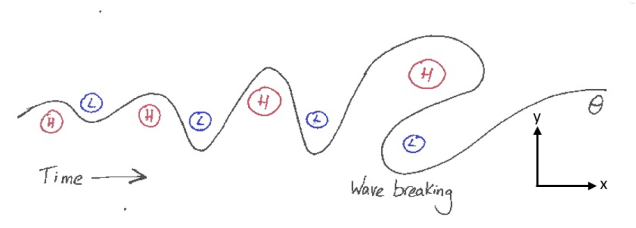
Up until recently cyclone clustering had been given little attention in terms of scientific research, despite it being a widely accepted phenomenon in the scientific community. With these events being such high risk events it is important to understand the atmospheric dynamics that are associated with these events; and this is exactly what we have been doing recently. In our new study we attempt to characterise cyclone clustering in several different locations and associate each different set of clusters with a different dynamical setup in the upper troposphere. The different locations we focus on are defined by three areas, one encompassing the UK and centred at 55°N. Our other two areas are 10° to the north and south of this (centred at 65°N and 45°N.) The previous study of Pinto et al. (2014) examined several winter seasons and found links between the upper-level jet, Rossby wave breaking (RWB) and the occurrence of clustering. RWB is the meridional overturning of air in the upper troposphere. It is identified using the potential temperature (θ) field on the dynamical tropopause, with a reversal of the normal equator-pole θ gradient representing RWB. This identification method is explained in full in Masato et al. (2013) and also illustrated in figure 2. We have greatly expanded on this analysis to look at all winter clustering events from 1979/1980 to 2014/2015 and their connection with these dynamical features.
Figure 2. Evolution of Rossby waves on the tropopause. RWB occurs when these waves overturn by a significant amount. H: High potential temperature; L: Low potential temperature (Priestley et al., 2017).
We find that when we get clustering it is accompanied with a much stronger jet at 250 hPa than in the climatology, with average speeds peaking at over 50 ms-1 (figures 3a-c). In all cases there is also a much greater presence of RWB in regions not seen from the climatology (Figure 3d). In figure 3a there is more RWB to the south of the jet, in figure 3b there is an increased presence on both the northern and southern flanks, and finally in figure 3c there is much more RWB to the north. The presence of this anomalous RWB transfers momentum into the jet, which acts to strengthen and extend it toward western Europe.
Figure 3. The dynamical setup for clustering occurring at (a) 65°N; (b) 55°N; and (c) 45°N. The climatology is shown in (d). Coloured shading is the average potential temperature on the tropopause, black contours are the average 250 hPa wind speeds and black crosses are where RWB is occurring.
The location of the RWB controls the jet tilt; more RWB to the south of the jet acts to angle it more northwards (figure 3a), there is a southward deflection when there is more RWB to the north of the jet (figure 3c). The presence of RWB on both sides extends it along a more central axis (figure 3b). Therefore the occurrence of RWB in a particular location and the resultant angle of the jet acts to direct cyclones to various parts of western Europe in quick succession.
In our recently published study we go into much more detail regarding the variability associated with these dynamics and also how the jet and RWB interact in time. This can be found at http://dx.doi.org/10.1002/2016GL071277.
This work is funded by NERC via the SCENARIO DTP and is also co-sponsored by Aon Benfield.
References
Della-Marta, P. M., Liniger, M. A., Appenzeller, C., Bresch, D. N., Köllner-Heck, P., & Muccione, V. (2010). Improved estimates of the European winter windstorm climate and the risk of reinsurance loss using climate model data. Journal of Applied Meteorolo
Kendon, M., & McCarthy, M. (2015). The UK’s wet and stormy winter of 2013/2014. Weather, 70(2), 40-47.
Masato, G., Hoskins, B. J., & Woollings, T. (2013). Wave-breaking characteristics of Northern Hemisphere winter blocking: A two-dimensional approach. Journal of Climate, 26(13), 4535-4549.
Pinto, J. G., Gómara, I., Masato, G., Dacre, H. F., Woollings, T., & Caballero, R. (2014). Large‐scale dynamics associated with clustering of extratropical cyclones affecting Western Europe. Journal of Geophysical Research: Atmospheres, 119(24).
Priestley, M. D. K., J. G. Pinto, H. F. Dacre, and L. C. Shaffrey (2017). The role of cyclone clustering during the stormy winter of 2013/2014. Manuscript in preparation.
Sulphate aerosol injection (SAI) is one of the geoengineering proposals that aim to reduce future surface temperature rise in case ambitious carbon dioxide mitigation targets cannot be met. Climate model simulations suggest that by injecting 5 teragrams (Tg) of sulphur dioxide gas (SO2) into the stratosphere every year, global surface cooling would be observed within a few years of implementation. This injection rate is equivalent to 5 million tonnes of SO2 per year, or one Mount Pinatubo eruption every 4 years (large volcanic eruptions naturally inject SO2 into the stratosphere; the Mount Pinatubo eruption in 1991 led to ~0.5 °C global surface cooling in the 2 years that followed (Self et al., 1993)). However, temperature fluctuations occur naturally in the climate system too. How could we detect the cooling signal of SAI amidst internal climate variability and temperature changes driven by other external forcings?
The answer to this is optimal fingerprinting (Allen and Stott, 2003), a technique which has been extensively used to detect and attribute climate warming to human activities. Assuming a scenario (G4, Kravitz et al., 2011) in which 5 Tg yr-1 of SO2 is injected into the stratosphere on top of a mid-range warming scenario called RCP4.5 from 2020-2070, we first estimate the climate system’s internal variability and the temperature ‘fingerprints’ of the geoengineering aerosols and greenhouse gases separately, and then compare observations to these fingerprints using total least squares regression. Since there are no real-world observations of geoengineering, we cross-compare simulations from different climate models in this research. This gives us 44 comparisons in total, and the number of years that would be needed to robustly detect the cooling signal of SAI in global-mean near-surface air temperature is estimated for each of them.
Figure 1(a) shows the distribution of the estimated time horizon over which the SAI cooling signal would be detected at the 10% significance level in these 44 comparisons. In 29 of them, the cooling signal would be detected during the first 10 years of SAI implementation. This means we would not only be able to separate the cooling effect of SAI from the climate system’s internal variability and temperature changes driven by greenhouse gases, but we would also be able to achieve this early into SAI deployment.
Figure 1: Distribution of the estimated detection horizons of the SAI fingerprint using (a) the conventional two-fingerprint detection method and (b) the new, non-stationary detection method.
The above results are tested by applying a variant of optimal fingerprinting to the same problem. This new method assumes a non-stationary background climate that is mainly forced by greenhouse gases, and attempts to detect the cooling effect of SAI against the warming background using regression (Bürger and Cubasch, 2015). Figure 1(b) shows the distribution of the detection horizons estimated by using the new method in the same 44 comparisons: 35 comparisons would require 10 years or fewer for the cooling signal to be robustly detected. This shows a slight improvement from the results found with the conventional method, but the two distributions are very similar.
To conclude, we would be able to separate and thus, detect the cooling signal of sulphate aerosol geoengineering from internal climate variability and greenhouse gas driven warming in global-mean temperature within 10 years of SAI deployment in a future 5 Tg yr-1 SAI scenario. This could be achieved with either the conventional optimal fingerprinting method or a new, non-stationary detection method, provided that the climate data are adequately filtered. Research on the effects of different data filtering techniques on geoengineering detectability is not included in this blog post, please refer to the article cited at the top for more details.
This work has been funded by the University of Reading. Support has also been provided by the UK Met Office.
Note: So how feasible is a 5 Tg yr-1 SO2 injection scenario? Robock et al. (2009) estimated the cost of lofting 1 Tg yr-1 SO2 into the stratosphere with existing aircrafts to be several billion U.S. dollars per year. Scaling this to 5 Tg yr-1 is still not a lot compared to the gross world product. There are practical issues to be addressed even if existing aircrafts were to be used for SAI, but the deciding factor of whether to implement sulphate aerosol geoengineering or not would likely be its potential benefits and side effects, both on the climate system and the society.
References
Self, Stephen, et al. “The atmospheric impact of the 1991 Mount Pinatubo eruption.” (1993).
Allen, M. R., and P. A. Stott. “Estimating signal amplitudes in optimal fingerprinting, Part I: Theory.” Climate Dynamics 21.5-6 (2003): 477-491.
Kravitz, Ben, et al. “The geoengineering model intercomparison project (GeoMIP).” Atmospheric Science Letters 12.2 (2011): 162-167.
Bürger, Gerd, and Ulrich Cubasch. “The detectability of climate engineering.” Journal of Geophysical Research: Atmospheres 120.22 (2015).
Robock, Alan, et al. “Benefits, risks, and costs of stratospheric geoengineering.” Geophysical Research Letters 36.19 (2009).
From 12th to 16th December 2016, the annual American Geophysical Union (AGU) Fall Meeting took place at the Moscone Centre in San Francisco. AGU remains the largest Earth and Space Science conference in the world with more than 25,000 scientists.
Overlooking the Poster Hall in Moscone South
At the 2016 Fall Meeting, I was one of around 8000 students who arrived in San Francisco to present one of the 15,000 posters that would be displayed over the course of the week. While I knew that AGU is one of the largest Earth science conferences, and had indeed spent hours on the plane fine-tuning my schedule to choose which of the ~200 hydrology sessions (let alone the meteorology sessions also related to my work) I would attend, the scope and diversity of the research presented throughout the week really sunk in when I stood on the mezzanine overlooking the poster hall on the first day of the conference.
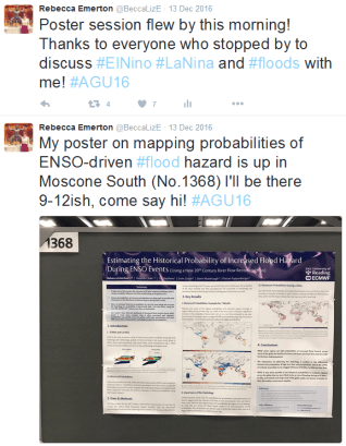
I was lucky enough to be awarded an AGU student travel grant in order to present my latest PhD research that I’ve been working on at the University of Reading, in collaboration with the European Centre for Medium-Range Weather Forecasts (ECMWF), and funded by NERC as part of the SCENARIO Doctoral Training Partnership. My work maps the historical probability of increased (or decreased) flood hazard across the globe during ENSO (El Niño and La Niña) events, using the first 20th Century ensemble river flow reanalysis, created at ECMWF as part of this work. But more on that another time!
Unlike other conferences I’d presented at, the poster sessions at AGU span half a day – while you are only expected to be there to discuss the work for two hours, it’s inevitable that you get caught up in discussion and I saw many presenters (myself included) who stuck by their poster for the full 4.5 hours! I thoroughly enjoyed my poster session, where several familiar faces dropped by for an update on my work, and others stopped to pose new questions and make a few suggestions for improvements to my maps (wait, why didn’t I think of that?!). As a student presenter, I could also register for the Outstanding Student Poster Award – which means that my poster was anonymously judged, and I will soon be receiving feedback on my poster and presentation – an opportunity I was excited about to make sure I continue to improve the way I communicate my research.
For me, some of the sessions that were highlights of the conference included ‘Global Floods: Forecasting, Monitoring, Risk Assessment and Socioeconomic Response‘, ‘Large-scale Climate Variability and its Impact on Hydrological Systems, Water Resources and Population‘, ‘Forecasting Hydrology at Continental Scale‘, ‘Transforming Hydrologic Prediction and Decision Making: Uncertainty’ and ‘ENSO Dynamics, Observations and Predictability in light of the 2015-2016 El Niño Event‘. With such a range of science being presented, there’s also plenty of opportunity (well, so long as you haven’t double- or triple-booked sessions in your schedule already!) to listen to talks outside of your own field – which is how I ended up in an 8am talk on operational earthquake forecasting and early warning. It was brilliant to learn about forecasting natural hazards outside of hydrology and meteorology!
There was also the social aspect that’s a big part of any conference – networking, networking and more networking! While it can be daunting, particularly at a conference of this size, to find and introduce yourself to scientists in your field whose work you’ve read but you’ve never met, I was pleased to first bump into some friendly faces who in turn introduced me to the new faces. Plus, it’s an AGU tradition that ‘AGU beer’ is served at 3.30pm sharp and the conference centre fills with groups of friends and colleagues in heated debates and discussions about anything from volcanoes to Jupiter’s magnetosphere.
It was impossible not to notice, however, the many more politically-themed conversations than would normally be overheard at such an event, as a result of uncertainty about the future of science in light of the recent US presidential election. While I was in the middle of research discussions at my poster, a ‘Stand up for Science‘ rally took place a few blocks away from the conference centre, where scientists donned lab coats and held signs – “stand up for science”, “ice has no agenda – it just melts” – protesting to raise awareness of the challenges, and to support science. You can read the Guardian article here.
All in all, AGU was a brilliant chance to present and discuss part of my research that I had just finished – it was certainly overwhelming and tough to choose which sessions to stop by (which meant I missed one or two presentations that sounded great), but I would recommend it for showcasing your work (and receiving feedback via the OSPA) and meeting scientists in your field that you wouldn’t normally bump into at conferences in Europe, especially if you can apply for one of AGU’s travel grants to help cover the costs of getting there.
P.S. You can watch presentations from the AGU Fall Meeting 2016 on the website.
Of course, I couldn’t fly all the way out to California and not find time to explore San Francisco a little.